

Abstract
Humans tend to avoid mental effort. Previous studies have demonstrated this tendency using various demand-selection tasks; participants generally avoid options associated with higher cognitive demand. However, it remains unclear whether humans avoid mental effort adaptively in uncertain and nonstationary environments. If so, it also remains unclear what neural mechanisms underlie such learned avoidance and whether they remain the same regardless of cognitive-demand types. We addressed these issues by developing novel demand-selection tasks where associations between choice options and cognitive-demand levels change over time, with two variations using mental arithmetic and spatial reasoning problems (males/females: 29:4 and 18:2). Most participants showed avoidance, and their choices depended on the demand experienced on multiple preceding trials. We assumed that participants updated the expected cost of mental effort through experience, and fitted their choices by reinforcement learning models, comparing several possibilities. Model-based fMRI analyses revealed that activity in the dorsomedial and lateral frontal cortices was positively correlated with the trial-by-trial expected cost for the chosen option commonly across the different types of cognitive demand. Analyses also revealed a trend of negative correlation in the ventromedial prefrontal cortex. We further identified correlates of cost-prediction error at time of problem presentation or answering the problem, the latter of which partially overlapped with or were proximal to the correlates of expected cost at time of choice cue in the dorsomedial frontal cortex. These results suggest that humans adaptively learn to avoid mental effort, having neural mechanisms to represent expected cost and cost-prediction error, and the same mechanisms operate for various types of cognitive demand.
SIGNIFICANCE STATEMENT In daily life, humans encounter various cognitive demands and tend to avoid high-demand options. However, it remains unclear whether humans avoid mental effort adaptively under dynamically changing environments. If so, it also remains unclear what the underlying neural mechanisms are and whether they operate regardless of cognitive-demand types. To address these issues, we developed novel tasks where participants could learn to avoid high-demand options under uncertain and nonstationary environments. Through model-based fMRI analyses, we found regions whose activity was correlated with the expected mental effort cost, or cost-prediction error, regardless of demand type. These regions overlap, or are adjacent with each other, in the dorsomedial frontal cortex. This finding helps clarify the mechanisms for cognitive-demand avoidance, and provides empirical building blocks for the emerging computational theory of mental effort.
- avoidance learning
- cognitive demand
- decision making
- mental effort
- model-based fMRI
- reinforcement learning
Introduction
Humans tend to avoid mental effort in various situations associated with many types of cognitive demand. When making complex decisions, humans tend to rely on heuristics instead of effortful reasoning (Tversky and Kahneman, 1974). Humans also discount reward values when mental effort is required (Botvinick et al., 2009; Massar et al., 2015; Chong et al., 2017), and expend physical effort to reduce mental effort (Risko et al., 2014). Moreover, exertion of mental effort causes fatigue effects on subsequent choice behavior (Blain et al., 2016). To clarify the precise nature of mental-effort avoidance in the absence of other factors affecting decisions, such as reward or physical effort, previous researchers developed the demand-selection task paradigm (Botvinick, 2007). In this paradigm, participants freely choose one of two cues associated with high and low cognitive demands. By using several variations of the task, researchers have demonstrated the generality of cognitive-demand avoidance, to the extent that potential confounders, such as the rate of errors or the time on task, could not fully explain (Kool et al., 2010).
In daily life, the cognitive demands of choice options encountered are likely to change over time. Work using this demand-selection task (Kool et al., 2010) has examined the condition where participants needed to learn the association between novel cues and stable demand levels in every task block, finding that most participants consistently avoided higher-demand options. However, it has yet to be experimentally demonstrated whether humans adaptively learn to avoid higher cognitive demand through experience in situations where demand levels are not stationary, i.e., when the association between cues and demand levels fluctuates and changes over time.
Moreover, if humans exhibit this kind of experience-based adaptive learned avoidance of mental effort, exploring its neural basis is of particular interest. A number of studies have identified neural correlates of the level of imposed cognitive demand (Botvinick et al., 2001; Duncan, 2010; Mansouri et al., 2017; Shenhav et al., 2017) or anticipated cognitive demand (Sohn et al., 2007; Krebs et al., 2012; Vassena et al., 2014), the avoidance rating of experienced cognitive demand (McGuire and Botvinick, 2010), or the mental effort-discounting of reward values (Botvinick et al., 2009; Massar et al., 2015; Chong et al., 2017). However, the results of these studies are not yet sufficient to understand the neural mechanisms for adaptive learned avoidance of mental effort. Significantly, the previous imaging studies did not examine brain activity during learned avoidance based on trial-by-trial experience.
Furthermore, to clarify general neural mechanisms for mental-effort avoidance (i.e., those which operate regardless of demand type), it is necessary to test more than one type of cognitive demand. The previous imaging studies on anticipation or avoidance of cognitive demand tested only a single type of cognitive demand in each study (Sohn et al., 2007; Botvinick et al., 2009; Krebs et al., 2012; Vassena et al., 2014; Massar et al., 2015; Chong et al., 2017). Therefore, it remains unclear whether the same neural mechanisms underlie avoidance of various types of cognitive demand.
To address these questions, we formed two hypotheses. First, we hypothesized that humans adaptively learn through experience to avoid an option that presently requires higher cognitive demand in the situation where the demand level of options changes over time. This learning process was assumed to be approximated by reinforcement-learning models in which the expected cost of mental effort is updated according to prediction error (PE). Second, we hypothesized that the expected cost estimated from the model is represented in the same brain regions regardless of the types of cognitive demands. To test these hypotheses, we developed two tasks requiring different cognitive-demand types where associations between choice options and cognitive-demand levels change over time. We fitted participants' choices using various models, conducted model comparisons, and explored brain regions representing the expected mental effort cost and cost-prediction error (CPE) through model-based fMRI analyses.
Materials and Methods
Participants
There were 33 participants (four females; mean age, 25.5 ± 5.4 years) in Experiment 1 and 20 participants (two females; mean age, 24.7 ± 6.2 years) in Experiment 2. Six participants took part in both experiments. We paid all participants equally with book store gift cards (worth ¥6000) for their participation. No participants were taking any medicine or had prior history of neuropsychiatric disorders. All participants were right-handed and native Japanese speakers. Informed written consent was obtained from all participants before the experiment. The present study was approved by the ethics committee of the Graduate School of Medicine, the University of Tokyo.
Behavioral tasks
We include a method summary for behavioral tasks and analyses in the Results, and here we describe all the details. We conducted two experiments. These had the same structure but used different types of problems requiring different kinds of cognitive activity (Fig. 1). Specifically, we used mental division (arithmetic) problems in Experiment 1 and mental cube-folding (spatial reasoning) problems in Experiment 2. For both experiments, we prepared problems with two levels of cognitive demand, i.e., high-demand and low-demand problems.
In Experiment 1, we required participants to divide a five-digit number by 7 and report whether the remainder was small (≤3) or large (≥4) via a button press with no time limitations. In low-demand problems, the dividend (e.g., 35426) consisted of two consecutive two-digit numbers that were multiples of 7 followed by a single one-digit number from 1 to 6. In contrast, the dividend of high-demand problems did not contain any numbers that were multiples of 7 in mental calculation processes (e.g., 48106). More specifically, the set of low-demand problems consisted of seven patterns for the digits representing ten-thousands and thousands (14, 21, 28, 35, 42, 49, 56, 63, 70), seven patterns for the digits representing hundreds and tens (7, 14, 21, 28, 35, 42, 49, 56, 63), and six patterns for the digits representing ones, and a combination of them was pseudorandomly selected in each trial. Meanwhile, dividends in higher-demand problems satisfying the above-mentioned rule were selected on each trial by using a pseudorandom function. The five-digit numbers and the answer choices were presented as gray characters on a black background.
In Experiment 2, we required participants to judge whether a concurrently presented 3D cube with three visible colored faces matched an unfolded cube with all six faces and colors (purple, red, yellow, green, sky blue, and deep blue), and report the answer via a button press with no time limitations. The difference between low-demand and high-demand problems was whether the three faces shown on the 3D cube were adjacent on the unfolded cube. There were in total 78 patterns (match, 39; nonmatch, 39) for low-demand problems and 120 patterns (match, 60; nonmatch, 60) for high-demand problems, and in each trial, one problem was pseudorandomly selected from these patterns with duplication permitted. The set of high-demand problems used was selected from all the possibilities so that the correct ratio was expected to be ≥0.8 based on the results of pilot experiments. The 3D and unfolded cubes and the answer choices (match, circle; nonmatch, cross) were presented on a white background. The locations of the answer choices (circle and cross), in either the left-bottom or right-bottom, were fixed for each participant and counter-balanced across participants.
In both Experiments 1 and 2, at the start of each trial, two arrow cues appeared, one on the left and the other on the right of the screen (via the overhead mirror). Participants were asked to choose one of them, without time restriction, to specify whether to solve the “left-arrow” problem or the “right-arrow” problem on that trial (without seeing the problem itself). Three seconds after participants chose one of the arrow cues, the chosen problem was presented in the center of the screen. Participants were asked to answer the problem (no time limitation), and when a choice was made by a button press, an intertrial interval started, followed by the next trial. The intertrial intervals were jittered: 2.5, 4, or 5.5 s. We asked participants to answer problems as fast and accurately as possible, giving weight to the accuracy. We further instructed the participants that if they felt unsure about their answer, they were asked to redo the mental calculation or cube-folding until they were sure. We did not provide correct/incorrect feedback to participants so as to minimize the possible effects of mistakes on the way participants made decisions.
The probability that a high-demand or low-demand problem appeared depended on whether participants chose the left-arrow cue or the right-arrow cue at the start of each trial, and the probabilistic associations between each of the cues and high-demand and low-demand problems changed over trials (Fig. 1B). Specifically, when programming the task, we divided the entire 180 trials into six blocks. In the first, third, and fifth blocks, the left and right arrow-cues were associated with low-demand problems in 80 and 20% of trials within each block, respectively. In the remaining (i.e., second, fourth, and sixth) blocks, the cue–demand associations were reversed, i.e., the left and right arrow-cues were associated with low-demand problems in 20 and 80% of trials within each block, respectively. The length (number of trials) of the first, third, and fifth block was 20, 30, or 40 trials; their order was pseudorandomized for each participant. The same was applied to the length of the second, fourth, and sixth block. Notably, participants were not informed of when the task entered a new block, or even of the existence of these different blocks.
In both Experiments 1 and 2, the low-demand and high-demand problems had very similar visual properties and the same task rule, so the differences between them were limited to the level of cognitive demand. We instructed the participants that there were two types of problems and the probabilities that the two types appeared varied across trials individually in the left-arrow problems and the right-arrow problems. As described above, the ratios of low-demand and high-demand problems in the left-arrow and right-arrow problems in each block were symmetric, i.e., either 80 and 20% or 20 and 80%. However, the moving average rates of the problem types were not generally symmetric, as shown in Figure 1B, and so we expected that the participants felt that the left and right probabilities of the two types varied individually as instructed. In the initial instruction about the two problem types, we did not explain that the difference between the two types was in the level of cognitive demands (but see below for our communications with participants during instruction and practice sessions).
Before scanning, participants received instructions and practiced the tasks for 5–20 trials in Experiment 1 and 30–60 trials in Experiment 2 to get acclimated to the tasks and recognize that there were two types of problems. During the practice session(s), we continued to give oral instructions to and accept questions from participants. After the practice session(s), we asked the participants to explain what they thought was the difference between the two types. When participants' reports reflected the actual difference in the problem content or when they said that they thought the difference was in the level of difficulty or largely similar things, we told them that we could not say the answer was correct or not. When the difference that participants reported was wildly incorrect, we told them that the answer was wrong and let them practice more, and when the participants subsequently reported things closer to reality, we (sometimes) said that the answer was not largely incorrect. Notably, to ensure that participants made their choices freely and without bias from us, we never told participants to avoid high-demand problems. Also, we instructed participants that their choices did not affect how fast they could finish the experiments so as to minimize the possible effects of this factor on participants' decision making.
In the scanner, in both Experiments 1 and 2, there were in total 180 trials, which were divided into four sessions, each consisting of 45 trials (note that these sessions were different from the abovementioned six blocks). In each session, when a participant completed (chose an arrow cue and answered the problem) up to the 10th, 20th, 30th, and 45th (i.e., the last) trial in the session in <160, 320, 480, and 750 (in Exp. 1) or 900 (in Exp. 2) s, respectively, a rest period was imposed until 160, 320, 480, and 750 (in Exp. 1) or 900 (in Exp. 2) s had passed so as to make the progression of trials as independent as possible from participants' choices. We instructed participants that the left and right probabilities of each type of problems would change continuously across sessions.
Image acquisition
We used a Siemens 3T Trio scanner (Brain Science Institute, Tamagawa University). When scanned, participants wore a head strap with memory foam to reduce their head movements. Participants viewed the experimental stimuli via a mirror reflecting the projector screen. Functional images were acquired in an ascending order and by using T2-weighted echo planar imaging sequence [repetition time (TR) = 2500 ms; echo time (TE) = 25 ms; field of view (FOV): 192 × 192 mm; in-plane resolution: 3 × 3 mm; acquisition matrix, 64 × 64; 42 slices with a slice thickness of 3.0 mm with no interslice gap]. In Experiment 1, ≥305 volumes were acquired, but just 305 were used for fMRI analysis in each of the four sessions for each participant. In Experiment 2, ≥365 volumes were acquired, but just 365 volumes were used for fMRI analysis in each of the four sessions for each participant. The first five scans in each session were discarded to allow for steady-state magnetization. We acquired high-resolution T1-weighted images using a MPRAGE sequence for all participants (TR = 2000 ms; TE = 1.98 ms; in-plane resolution, 1 × 1 mm; slice thickness, 1 mm).
Experimental design and statistical analysis
Behavioral analysis.
In both experiments, one participant was excluded from analysis due to low correct rates (<80% for both types). We first tested whether each participant chose the opposite option (left or right) after solving a high-demand problem more frequently than after solving a low-demand problem. Specifically, we conducted a χ2 test on the contingency table consisting of the problem types (high or low demand) of the previous trials and the choices (same or opposite) of the current trials for each participant, and judged that s/he avoided high-demand problems if the frequency was significantly different (p < 0.01) and the adjusted standardized residuals were negative in the high × same and low × opposite cells of the contingency table. We next analyzed the effect of the demand experienced two trials prior (i.e., the trial before the previous trial) on the choice at the current trial for participants who showed avoidance of high-demand problems (judged through the χ2 test as described above). Specifically, we compared the proportion that the k-th choice was the same as the (k − 2)-th choice (k = 3, 4, …, 180) between the cases where the experienced demand at the (k − 2)-th trial was high or low by using a paired t test as a planned comparison, for each case sorted by the (k − 1)-th choice (same as or opposite from the (k −2)-th) and the (k − 1)-th experienced demand (high or low). We sorted the data by the (k − 1)-th choice and demand because otherwise spurious dependence could appear, i.e., the rate that the k-th choice was the same as the (k − 2)-th choice could differ depending on the (k − 2)-th demand even if choice was made depending solely on the choice and demand on the previous trial. It was generally rare that participants chose the opposite side after experiencing low demand, and there were participants who did not have data for the cases that included such a pattern (Fig. 2, crosses). Those unpaired data were omitted from the t test. As a measure of the effect size, we reported Cohen's d calculated as follows:
 where μ1, μ2 and s1, s2 are the means and sample SDs of each set of the paired data, respectively. The SEM was calculated by dividing the SD [defined with
  (Figs. 2, 8) or
  (otherwise)] by
  , where n was the number of data included.
Model fitting, comparisons, simulations, and analyses of simulated behavioral data.
We fitted the choices of the participants judged to have avoided high-demand problems in the χ2 test using PE-based models (O'Doherty et al., 2007; Daw, 2011). We assumed that participants retained the expected cost (ExpectedCost) of mental effort for the left-arrow and right-arrow problems [ExpectedCostleft(k) and ExpectedCostright(k) (k = 1, 2, …, 180: trials)]. At each trial k, either the left or right arrow was assumed to be chosen with the probabilities Pleft(k) and Pright(k), respectively, depending on the expected cost, expressed as follows:

 where β was a free parameter called the inverse temperature. If β was positive, the option with lower ExpectedCost was more frequently chosen, and the size of β represented the degree of exploitation over exploration. After solving a problem, the CPE was assumed to be calculated as follows: CPE(k) = ActualCost(k) − ExpectedCostChoice(k), where ActualCost(k) was the actual cost of the solved problem, and Choice(k) was Left or Right depending on which was chosen. As ActualCost, we considered five cases: (1) time spent solving the problem (solve time; in seconds) in individual trials [PE-Solve-Time (ST) model]; (2) demand level of the problem; more specifically, 1 and 0 for high-demand and low-demand problems, respectively [PE-High-Low (HL) model]; (3) incorrect solving; more specifically, 1 and 0 for incorrect and correct solving, respectively (PE-Incorrect-Correct (IC) model; (4) sum of (1) and (3), with a weighting parameter for (3) (wincorrect), i.e., solve-time + wIncorrect · incorrect-solving (PE-ST-IC model); and (5) sum of (2) and (3), with a weighting parameter for (3) (wincorrect), i.e., demand-level + wIncorrect · incorrect-solving (PE-HL-IC model).
ExpectedCost for the chosen option was then assumed to be updated as follows: ExpectedCostChoice(k)(k + 1) = ExpectedCostChoice(k)(k) + α · CPE(k), where α was a free parameter representing the learning rate. ExpectedCost for the unchosen option was assumed to be unchanged. ExpectedCost for the option chosen at the first trial [ExpectedCostChosen(1)] was assumed as follows, depending on the five cases for ActualCost: (i) the mean solve time across all the trials in case (1) above (i.e., for the PE-ST model); (ii) 0.5 in case (2) (for the PE-HL model); (iii) the mean incorrect rate in case (3) (for the PE-IC model); (iv) sum of (i) and (iii) with the weighting parameter for (iii) in case (4) (for the PE-ST-IC model); and (v) sum of (ii) and (iii) with the weighting parameter for (iii) in case (5) (for the PE-HL-IC model).
ExpectedCost for the unchosen option at the first trial [ExpectedCostunchosen(1)] was assumed to be either a free parameter or equal to ExpectedCostChosen(1) (i.e., we examined both cases for each of the five cases for ActualCost): in total 5 × 2 = 10 models). Because the practice session(s) was rather short and we continued to give oral instructions to and accept questions from participants during the practice session(s), we considered it inappropriate to use performance measures during the practice session(s) for the initial values, and therefore we instead set the initial values as above.
In addition to these cost-based PE models, we also considered a PE model assuming that rest time in the scanner was a reward (ActualReward) for participants and they made choices based on the expectation of this reward (ExpectedReward) and updated ExpectedReward by reward PE (RPE; i.e., participants may have tried to choose low-demand problems so as to maximize “inactive time”). In this model, referred to as the PE-Rest model, ActualCost, ExpectedCost, and CPE were replaced with ActualReward, ExpectedReward, and RPE, respectively, and also β was replaced with −β. ActualReward was assumed to be the rest time (in seconds) from problem answer in the k-th trial to arrow presentation in the k + 1-th trial or to the end of session when the k-th trial was the last trial in the session. ExpectedRewardchosen(1) and ExpectedRewardunchosen(1) were assumed to be 4 s, given that the intertrial interval was 2.5, 4, or 5.5 s. We further considered a model combining this PE-Rest model and the best of the 10 cost-based PE models (which was the PE-HL model with ExpectedCostunchosen(1) = ExpectedCostChosen(1): see Results). In this model, referred to as the PE-HL-Rest model, ExpectedCost and ExpectedReward were assumed to be updated with individual learning rates (αcost and αreward), and choice was made based on the expected value that combined the expected cost and reward in a softmax manner with an inverse temperature β. The expected value was expressed as follows: ExpectedValueX(k) = wreward · ExpectedRewardX(k) − ExpectedCostX(k), where X was Left or Right and wreward was a free weighting parameter. The values of ExpectedReward and ExpectedCost at the first trial were assumed to be the same as those in the PE-Rest model and the PE-HL model with ExpectedCostunchosen(1) = ExpectedCostChosen(1).
In addition to the PE models, we also examined probabilistic Win-Stay-Lose-Shift (pWSLS) models, in which Win or Lose was followed by a selection of the same or different option, respectively, with exceptions with probability p that was a free parameter. We further examined full probabilistic-selection (PS) models, in which Win or Lose was followed by a selection of the same option with probabilities a and b, respectively, which were free parameters. For either type of model, Win and Lose were defined in two ways: (1) experiences of low-demand and high-demand problems, respectively (pWSLS-HL model and PS-HL model), or (2) solving correctly and incorrectly, respectively (pWSLS-IC model and PS-IC model).
For each of these models, we explored a set of free parameters that maximized the log-likelihood, expressed as follows:
 for each participant by using an optimization function (fminsearch) of the Matlab Optimization Toolbox and also a grid approach [more specifically, we conducted both exploration, using fminsearch assuming a set of initial parameters, and direct calculation of logL at various parameter values (grid points), and combined the results: see the codes for the analysis that is planned to be uploaded to a public database after publication]. For the pWSLS and PS models, Pchoice(1) was assumed to be 0.5. To compare the goodness of fit of each model while taking into account the penalty for a larger number of parameters, we calculated the Bayesian information criterion (BIC) as follows: BIC = −2 logL + qlog(180), where q was the number of free parameters.
Using the best-BIC PE model [PE-HL model with ExpectedCostunchosen(1) = ExpectedCostChosen(1); see Results], pWSLS-HL model, and PS-HL model, we performed simulations of task execution (180 trials) with the best-fit parameters for each individual demand-avoiding participant in each experiment. Specifically, for each demand-avoiding participant (judged based on the effects of the experienced demand at the previous trial through the above-mentioned χ2 test) in each experiment, we extracted the best-fit parameters for each of the three models. Then, using these parameters and the actual sequences of low-demand and high-demand problems for the left-arrow and right-arrow cues used in the experiments, we generated 180 (number of trials) choices 100 times (i.e., performed 100 simulation runs) by using different sets of pseudorandom numbers in Matlab. We then analyzed the effect of the demand experienced two trials prior on the choice at the current trial in the pooled simulated choices for each participant. Specifically, we calculated the proportion that the k-th choice was the same as the (k − 2)-th choice when the (k − 2)-th demand was high or low, for each case sorted by the choice and demand on the (k − 1)-th trial, in the pooled simulated choices [178 (the initial two trials were omitted from the total 180 trials) × 100 = 17,800 simulated choices] corresponding to each participant.
Functional imaging analysis.
We used SPM8 (http://www.fil.ion.ucl.ac.uk/spm/) for fMRI data processing and analysis. We realigned the volumes to the first images using a six-parameter rigid-body transformation. We corrected timing differences for each slice and normalized individual images. We applied a Gaussian kernel with a full-width at half-maximum of 8 mm for spatial smoothing. After excluding six participants from Experiment 1 and three participants from Experiment 2 with >3 mm head movements from those who met the performance criterion and showed avoidance of high-demand problems (see Results), we conducted general linear model (GLM) analysis of BOLD data (Exp. 1, n = 21; Exp. 2, n = 15). As pointed out by Mumford et al. (2015), when multiple parametric modulations exist for the regressor at the same time, SPM8 performs orthogonalization by default. We turned off this default operation by commenting out line 228 of spm_get_ons.m and lines 277–279 of spm_fMRI_design.m, which call spm_orth.m, in reference to http://imaging.mrc-cbu.cam.ac.uk/imaging/ParametricModulations (but the line numbers that were commented out differed from those described on this website). All individual and group analyses in each experiment were done at the whole-brain level.
At the individual level, we examined the following three GLMs (Fig. 3) designed to explore the correlates of ExpectedCost for the chosen option (referred to as ExpectedCostChosen) and the CPE, adjusted for the response time for choosing an arrow (referred to as RTchoice), actual demand level of the problem (referred to as problem-demand), and solve time. These GLMs included the regressors at arrow-cue presentation with parametric modulations by ExpectedCostChosen (derived from the best-BIC PE model; see Results) and RTchoice, regressors with the duration from problem presentation to answer with parametric modulations by problem-demand (0 and 1 for low-demand and high-demand problems, respectively) and solve time, regressor with parametric modulation by CPE at the time of problem presentation (GLM1), midpoint between problem presentation and answer (GLM2), or time of answer (GLM3), and regressors for motor response (at both arrow choice and answer in GLM1 and GLM2 and only at arrow choice in GLM3) and head movements. We also considered variants of GLM1, which are described in Results. For each of these GLMs, we convolved each regressor with the SPM8's canonical hemodynamic response function and performed one-sample t tests for individual maps for the regressor(s) of interest across 21 and 15 participants in Experiments 1 and 2, respectively. We calculated the variance inflation factor (VIF) using the Canlab Matlab toolboxes (https://github.com/canlab/CanlabCore) and judged whether collinearity of the regressor of interest was at a tolerable level considering that 5 or 10 is typically used as a cutoff value of VIF for the collinearity issue (Mumford et al., 2015).
At the group level, we reported correlates detected by GLM1–GLM3 in each experiment with a threshold of cluster-level familywise error (FWE) corrected p < 0.05 and voxel-level uncorrected p < 0.001 for the cases where at least one cluster was found with this threshold, or more specifically, for the positive correlates of ExpectedCostChosen in GLM1–GLM3 in both experiments, negative correlates of ExpectedCostChosen in GLM1–GLM3 in Experiment 1, positive correlates of CPE in GLM1–GLM3 in both experiments, and negative correlates of CPE in GLM1 and GLM3 in Experiment 2. For the other cases where results for individual experiments were reported, or more specifically, for the negative correlates of ExpectedCostChosen in GLM1–GLM3 in Experiment 2 and negative correlates of CPE in GLM1–GLM3 in Experiment 1 and in GLM2 in Experiment 2, we reported correlates with a threshold of voxel-level uncorrected p < 0.001 with voxel-size of ≥5 if we found any.
To detect common regions in the correlates found in Experiments 1 and 2, we conducted conjunction analyses, to which we applied a binary mask. We used two masks with different thresholds: the strict mask and the relaxed mask. The strict mask consisted of common voxels between the results of Experiments 1 and 2 with the threshold of cluster-level FWE corrected p < 0.05 and voxel-level uncorrected p < 0.001. The relaxed mask consisted of common voxels with the threshold of voxel-level uncorrected p < 0.01 (which mask was used for which analyses is described in Results and tables; the relaxed mask was used when no cluster was detected with the threshold of the strict mask in either experiment or no cluster was detected as a result of conjunction analysis with the strict mask). We then reported correlates detected in the masked conjunction analyses with a threshold of cluster-level uncorrected p < 0.05 and voxel-level uncorrected p < 0.001.
Results
Behavioral tasks and analyses
We conducted two experiments. These had the same task structure but used different types of problems that imposed different kinds of cognitive demand (Fig. 1A). In Experiment 1, we used mental arithmetic problems. We asked participants to divide a five-digit number by 7 and report whether the remainder was small (≤3) or large (≥4). In Experiment 2, we used spatial reasoning (mental cube-folding) problems. We asked participants to judge whether a 3D cube with three visible colored faces matched a concurrently presented unfolded cube or not. For both experiments, we prepared two sets of problems that required different levels of cognitive demand, i.e., low-demand problems and high-demand problems. In Experiment 1, the dividend in low-demand problems (e.g., 35426) consisted of two consecutive two-digit numbers that were multiples of 7 followed by a single one-digit number from 1 to 6. Meanwhile, the dividend in high-demand problems (e.g., 48106) did not contain any numbers that were multiples of 7. In Experiment 2, the difference between low-demand and high-demand problems was whether the three faces shown on the 3D cube were neighboring on the unfolded cube. In both experiments, the probability that a high-demand or low-demand problem appeared at each trial depended on a cue that participants chose at the start of the trial: there were two cues, the left and right arrows, and the probabilistic associations between each of the cues and high-demand and low-demand problems changed across trials, such as shown in Figure 1B. After participants chose a cue, a problem, either high or low demand, was presented, and they were asked to answer it. There was no time limit for response.

Behavioral paradigm. A, Participants chose an arrow cue at the start of each trial. After the choice, a problem was presented. In Experiment 1 (Exp. 1), the problem was mental arithmetic: to divide a five-digit number by 7 and report whether the remainder was small or large. In Experiment 2 (Exp. 2), the problem was spatial reasoning: to judge whether a 3D cube matched an unfolded cube. In both experiments, there were high-demand problems and low-demand problems, whose presentation rates were associated with the arrow cues and varied over time. B, An example of the presentation rates of low-demand problems (moving average of latest 5 trials) associated with the left arrow-cue (light gray) and the right arrow-cue (dark gray).
There were 33 participants (four females; mean age, 25.5 ± 5.4 years) in Experiment 1 and 20 participants (two females; mean age, 24.7 ± 6.2 years) in Experiment 2. Six participants took part in both experiments. Most of the participants were males, so the results cannot with certainty be generalized to females. The response time for choosing an arrow cue (RTchoice) was 0.95 ± 0.08 s (mean ± SEM) in Experiment 1 and 1.25 ± 0.21 s in Experiment 2. The mean correct answer rates for high-demand and low-demand problems were 0.94 ± 0.008 (mean ± SEM) and 0.98 ± 0.010, respectively, in Experiment 1, and 0.92 ± 0.024 and 0.99 ± 0.004 respectively, in Experiment 2. In both experiments, correct answer rates for low-demand problems were higher than those for high-demand problems on average (paired t test, t(32) = −3.0, p = 4.9 × 10⁻³, in Exp. 1; t(19) = −2.7, p = 1.3 × 10⁻², in Exp. 2). The mean solve times (i.e., times for problem solving) for high-demand and low-demand problems were 10.00 ± 0.70 s (mean ± SEM) and 1.86 ± 0.09 s, respectively, in Experiment 1, and 12.44 ± 1.13 s and 4.60 ± 0.32 s, respectively, in Experiment 2. In both experiments, participants took longer for high-demand problems on average (paired t test, t(32) = 12.5, p = 8.1 × 10⁻¹⁴, in Exp. 1; t(19) = 8.3, p = 1.1 × 10⁻⁷, in Exp. 2). To ensure the quality of data used, we set a performance criterion for inclusion. Specifically, we assumed a participant faithfully executed the problems if the correct answer rate was ≥0.8 for either low-demand or high-demand problems. As a consequence, one participant in each experiment was excluded from the following analyses.
As an initial analysis of the participants' learning and choice behavior, we inferred whether each participant learned to avoid high-demand problems from the dependence of choices on the previous trials. We reasoned that participants wanting to avoid high-demand problems (whether consciously or not) would stay at the same side (left or right) if a low-demand problem appeared in the previous trial but would rather switch to the opposite side if a high-demand problem appeared. We thus examined whether such a bias existed by conducting a χ2 test [on 2 × 2 factors: problem types (high or low demand) in the previous trial × choice (same side or opposite side) in the current trial]. In the results, significant bias (p < 0.01) existed in 26 of 32 (81.3%) and 17 of 19 (89.5%) participants in Experiments 1 and 2, respectively. Among these cases, 24 of 32 (75.0%) and 17 of 19 (89.5%) participants in Experiments 1 and 2, respectively, showed avoidance of high-demand problems. This indicates that these participants (i.e., the majority) learned to avoid high-demand problems in the situation where the probabilistic associations between cues and demand levels changed over time. Overall, these demand-avoiding participants in Experiments 1 and 2 experienced low-demand problems in 63.6 ± 1.0% (mean ± SEM) and 64.6 ± 1.2%, respectively, and chose the same option as in the previous trial in 74.9 ± 2.1% and 79.5 ± 1.8% (in Trials 2–180), respectively. On the other hand, the remaining two participants in Experiment 1 had the opposite bias, indicating that this minority of participants learned (chose) to seek high-demand problems.
Next, we analyzed whether the choices of the demand-avoiding participants as judged above depended also on the demand experienced two trials before the present trial, i.e., in the trial before the previous trial. The paired bars in Figure 2 show the proportions that the choice at the k-th trial was the same as the choice at the (k − 2)-th trial when the demand experienced at the (k − 2)-th trial was high (left bar) or low (right bar), for each case sorted by the choice and demand at the (k − 1)-th trial in Experiment 1 (Fig. 2Aa–d) and Experiment 2 (Fig. 2Ba–d). As shown in the figure, the proportion that the k-th choice was the same as the (k − 2)-th choice was significantly higher when the demand experienced at the (k − 2)-th trial was low than when it was high, with medium-to-large effect sizes, in two cases in Experiment 1 (Fig. 2Aa; p = 0.01, d = 0.73, t(23) = 2.89; Fig. 2Ab; p = 0.02, d = 0.46, t(23) = 2.59) and in two cases in Experiment 2 (Fig. 2Ba; p < 0.01, d = 1.27, t(16) = 4.9; Fig. 2Bc; p = 0.01, d = 1.13, t(16) = 2.98). In this way, in both experiments, the choices of the demand-avoiding participants did depend on the demand experienced two trials prior.

Effects of the experienced demand at two trials before on the current choice. The paired bars indicate the across-participants average proportions that the current (k-th) choice was the same as the choice at two trials before [(k− 2)-th] when the experienced demand at the (k − 2)-th trial was high (left bar) or low (right bar), for each case sorted by the choice at the (k − 1)-th trial [same as (a, b) or opposite (c, d) from the (k − 2)-th choice] and the experienced demand at the (k − 1)-th trial [high (a, c) or low (b, d)] in Exp. 1 (n = 24; A) or Exp. 2 (n = 17; B). The average was taken across the participants who were judged as demand-avoiding based on the effects of the experienced demand at the previous trial (see Results). The error bars indicate the mean ± SEM. The dots connected by lines indicate the data of individual participants who had paired data, while the crosses indicate the data of individual participants who lacked one of the paired data; both types of participants were included in the calculation of the average indicated by the bar heights. The paired data, represented by the dots, were compared by paired t test, and the cases indicated by asterisk were significant (p < 0.05): Aa, p = 0.01, d = 0.73, t(23) = 2.89; Ab, p = 0.02, d = 0.46, t(23) = 2.59; Ba, p < 0.01, d = 1.27, t(16) = 4.89; Bc, p = 0.01, d = 1.13, t(16) = 2.98.
Detailed analyses of learning and choice behavior
To analyze learning and choice behavior in detail, we fitted the choices using PE-based models (O'Doherty et al., 2007; Daw, 2011), considering that PE-based models have been suggested to be able to approximate reinforcement learning of reward values (McClure et al., 2003; O'Doherty et al., 2003; Daw et al., 2006) as well as avoidance learning of pain (Seymour et al., 2004; Roy et al., 2014; Zhang et al., 2016), physical-effort cost (Skvortsova et al., 2014), or sustained effort (selecting circles on the screen) concurrently with reward learning (Scholl et al., 2015). In particular, we assumed that (1) participants had (whether consciously or not) expectations of the cost of mental effort, referred to as the ExpectedCost below, needed to solve a left or right problem (denoted by ExpectedCostleft and ExpectedCostright), (2) participants chose either the left or the right problem according to ExpectedCostleft and ExpectedCostright in a “softmin” manner, i.e., avoided an option with a higher ExpectedCost with a higher probability, and (3) the ExpectedCost for the chosen option (denoted by ExpectedCostChosen) was updated according to the CPE: ActualCost − ExpectedCostChosen, where the ActualCost was the cost actually experienced.
Given that participants took much longer times for high-demand problems than for low-demand problems on average as shown above, it is possible that the time spent to solve the problem constituted ActualCost, while it is also conceivable that ActualCost directly reflected the demand level of the problem itself. Moreover, because the correct answer rates also differed between the low-demand and high-demand problems, incorrect solving could also constitute or contribute to ActualCost, even though the incorrect answer rates were rather low and we did not provide correct/incorrect feedback to participants. With these considerations, we considered the following five cases for constituent(s) of ActualCost: (1) time spent solving the problem (solve time) in individual trials [referred to as the PE-Solve-Time(ST) model]; (2) demand level of the problem; more specifically, 1 and 0 for high-demand and low-demand problems, respectively [PE-High-Low(HL) model]; (3) incorrect solving; more specifically, 1 and 0 for incorrect and correct solving, respectively [PE-Incorrect-Correct(IC) model]; (4) sum of (1) and (3), with a weighting parameter for (3) (PE-ST-IC model); and (5) sum of (2) and (3), with a weighting parameter for (3) (PE-HL-IC model).
For each of these five cases, we considered two models assuming that ExpectedCost for the unchosen option (ExpectedCostunchosen) at the first trial was either a free parameter or a value equal to ExpectedCostChosen, resulting in 5 × 2 = 10 models.
We fitted these models to the participants' choices, individually for each participant who showed avoidance of high-demand problems (as judged by the χ2 test above), by exploring parameters that maximized the log-likelihood. We then compared the fitted models according to the BIC. As a result, the model assuming case (2) ActualCost [i.e., the PE-High-Low(HL) model] and ExpectedCostunchosen = ExpectedCostChosen at the first trial had the best (i.e., least) BIC score for most of the participants in both experiments (23 of 24 in Exp. 1; 14 of 17 in Exp. 2; Fig. 4A; Table 1; hereafter we refer to this model as the PE-HL model). This result indicates that mental-effort cost in our experiments was experienced and/or registered as (nearly) binary variables corresponding to the binary demand levels of the problems, rather than variables reflecting the solve time or mistakes (we will return to this later). An example of the fit by this model is shown in the red solid line in Figure 5, and the results of all the analyzed participants in Experiments 1 and 2 are shown in Figures 6 and 7, respectively.

GLMs and regressors used in the fMRI analyses. We explored the correlates of the expected cost of mental effort for the chosen option (ExpectedCostChosen) and the CPE estimated in the model by using three GLMs (GLM1–GLM3), which assumed three different possibilities regarding the time of CPE generation/representation. Each of these GLMs included the regressors at arrow-cue presentation with nonorthogonized parametric modulations by ExpectedCostChosen and RTchoice, regressors starting at problem presentation and having the duration of solve-time with nonorthogonized parametric modulations by demand level (1 and 0 for high-demand and low-demand problems, respectively) and solve time, regressors for motor response at both arrow choice and answer (GLM1 and GLM2) or at arrow choice (GLM3), regressors for head movements (not illustrated here), and regressor at problem presentation (GLM1), midpoint between problem presentation and answer (GLM2), or answer (GLM3) with parametric modulation by CPE.

BIC scores of the models fitted to the choices of demand-avoiding participants. A, The bars indicate the mean ± SEM of BIC scores for 10 variants of PE models in Experiments 1 (Exp. 1) and 2 (Exp. 2). The horizontal axis indicates the 10 PE models: five assumptions on ActualCost [Solve-Time (ST), High-Low (HL), Incorrect-Correct (IC), ST-IC, and HL-IC: see the Results for details] × 2 assumptions on ExpectedCostunchosen(1) [free parameter (light-gray bars) or equal to ExpectedCostChosen(1) (dark-gray bars)]. The black dots connected with the lines indicate individual demand-avoiding participants. B, Results for the additionally considered PE models that regarded the rest time in the scanner as reward for participants. C, Results for pWSLS models and PS models.
BIC scores and best-fit parameters of the models fitted to the choices of demand-avoiding participants

Example of participant's choices and choice probability predicted by the PE-HL model. Short vertical bars at the top and bottom indicate participant's left and right choices, respectively, with dark or light gray indicating that high-demand or low-demand problems were experienced, respectively. The black dashed line in the middle indicates the left–right difference in the presentation rates (moving average of latest 5 trials) of low-demand problems plotted against the left scale. The blue and red solid lines indicate the participant's actual left-choice rate (moving average of latest 5 trials) and the left-choice probability predicted by the PE-HL model plotted against the blue and red scales on the right, respectively. The best-fit parameters for this participant (in Exp. 1) were as follows: [learning rate, inverse temperature] = [0.68, 3.62]).

Results of model fitting for all the participants who showed avoidance in Experiment 1. The configurations are the same as those of Figure 5.

Results of model fitting for all the participants who showed avoidance in Experiment 2. The configurations are the same as those of Figure 5.
We additionally examined two more PE models that assumed that the rest time in the scanner was reward for participants and they made choices based on the expectation of this reward (referred to as the PE-Rest model) or on the expectations of both this reward and the mental-effort cost, which was assumed to be 0 and 1 for low-demand and high-demand problems, respectively, inheriting the assumption of the PE-HL model that gave the best BIC score (referred to as the PE-HL-Rest model). However, these models gave larger (i.e., worse) BIC scores than the PE-HL model in almost all cases (except for one participant in Exp. 1 for both PE-Rest and PE-HL-Rest models; Fig. 4B).
We also examined models having different structures from the PE models. In particular, we considered a pWSLS model, in which Win or Lose was followed by a selection of the same or different option, respectively, with exceptions with a certain probability that was a free parameter. Win and Lose were defined in two ways: (1) experiences of low-demand and high-demand problems, respectively (pWSLS-HL model), or (2) solving correctly and incorrectly, respectively (pWSLS-IC model). As a result, for either type of pWSLS models, participants for whom the given type of pWSLS model gave smaller (i.e., better) BIC scores than the PE-HL model (i.e., the best-BIC PE model) were outnumbered by those who had the opposite pattern (pWSLS-HL model: 14 of 24 in Exp. 1; 16 of 17 in Exp. 2; pWSLS-IC model: 20 of 24 in Exp. 1; 15 of 17 in Exp. 2; Fig. 4C). We further considered a full probabilistic selection (PS) model, in which Win or Lose was followed by a selection of the same or a different option with arbitrary probabilities that were free parameters, with the same two definitions of Win and Lose as above (PS-HL model and PS-IC model). As a result, the number of participants for whom the PS-HL model gave a smaller (better) BIC score than the PE-HL model was comparable to the number of those who had the opposite pattern in Experiment 1 [12 participants for each; though the average BIC score across participants was smaller (better) in the PS-HL model], and the PS-HL model gave a smaller (better) BIC score than the PE-HL model in a large number of participants in Experiment 2 (13 of 17; Fig. 4C). The PS-IC model gave larger (worse) BIC scores than the PE-HL model in most participants (23 of 24 in Exp. 1; 15 of 17 in Exp. 2; Fig. 4C).
As seen above, in terms of BICs, while the PE-HL model gave better fit than the pWSLS models and the PS-IC model, the PS-HL model outperformed the PE-HL model. Nevertheless, because the PS models, as well as the pWSLS models, assume that choice depends solely on the outcome of the previous trial, these models were expected to be unable to explain the observed considerable dependence of the actual choices on the experienced demand at two trials before (Fig. 2). To confirm this, we performed simulations of task execution by the PS-HL and pWSLS-HL models, as well as the PE-HL model, with the best-fit parameters for each individual demand-avoiding participant and actual demand sequences (high or low for the left and right arrow-cues) used for the participant in the experiments. We performed 100 simulation runs of task execution (180 trials) for each demand-avoiding participant in each experiment, and examined the proportions that the k-th choice was the same as the (k − 2)-th choice when the (k − 2)-th demand was high or low, sorted by the (k − 1)-th choice and demand, in the pooled simulated choices corresponding to each participant (178 × 100 = 17,800 simulated choices: see Materials and Methods). As expected, dependence of the current choice on the demand at two trials before hardly appeared in the cases of the PS-HL and pWSLS-HL models, in contrast to the case of the PE-HL model (Fig. 8). In this way, although the PS-HL model gave good fit in terms of BIC scores, this model could not adequately explain the considerable dependence on multiple trials back observed in the actual choices, which could potentially be captured by the PE-HL model. Therefore, in the following we present model-based fMRI analyses by using the results of fitting by the PE-HL model.
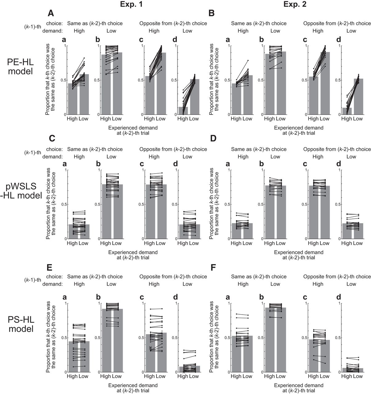
Effects of the experienced demand at two trials before on the current choice in pooled simulated choices. A, B, The dots connected by lines indicate the proportions that the k-th choice was the same as the (k − 2)-th choice when the (k − 2)-th demand was high (left) or low (right), sorted by the (k − 1)-th choice and demand (a–d), in pooled simulated choices corresponding to each demand-avoiding participant, which were generated by performing 100 simulation runs of task execution (180 trials) in Experiment 1 (Exp. 1; A) or Experiment 2 (Exp. 2; B) with actual demand sequences (high or low in the left or right) used for the participant by the PE-HL model with best-fit parameters for the participant. The bars indicate the average of the proportions corresponding to individual participants, and the error bars indicate the mean ± SEM. C–F, Same as A and B except that the pWSLS-HL model (C, D) or the PS-HL model (E, F) was used instead of the PE-HL model.
fMRI analyses
We searched the whole brain for regions where changes in hemodynamic response for the presentation of the left or right arrow-cue were positively or negatively correlated with the ExpectedCost for the chosen option (ExpectedCostChosen). We also searched for regions correlated with the CPE. Regarding the time of CPE generation, there were multiple possibilities. To see this, we need to return to the result of model fitting that the PE-HL model assuming binary costs gave the best BIC among the PE models. As described before, this result indicates that mental-effort cost in our experiments was experienced and/or registered as (nearly) binary variables corresponding to the binary demand levels of the problems, rather than variables reflecting the solve time or mistakes. Looking more closely, this would involve (at least) two possibilities. The first possibility is that the demand level itself was registered as “actual cost” and used to update the expected cost, potentially even before the cost was experienced (i.e., before the problem was solved). The second possibility is that the experienced cost at the time of answer was in fact more closely approximated by binary variables than by the solve time in our experiments. Although response time is generally thought to relate to subjective difficulty, it is possible that the within-participant variances of the solve time for the problems of the same demand types in our experiments were due in a large part to factors that did not linearly relate to the experienced cost. For example, participants might sometimes solve a problem sluggishly so that solve time was large but experienced cost was not large: even though they were asked to solve as fast and accurately as possible, how well participants complied with this instruction was somewhat elusive given that there was no time limitation and no feedback/penalty, and also participants' mood could fluctuate during the experiment so as to modulate the solve time and experienced cost in potentially different or nonlinearly related ways.
If the first possibility mentioned above holds, CPE may be generated at the time of problem presentation (or soon after it) because the binary demand level of the problem could be recognized almost instantaneously, although CPE could also be represented at the time of answer if the neural process for updating the expected cost could operate only after the process for problem-solving was ended. On the other hand, if the second possibility mentioned above holds, CPE would be generated at the time of answer. There was yet another possibility that CPE was generated at a time between problem presentation and answer. Therefore, by using separate GLMs (Fig. 3, GLM1–GLM3), we examined three possibilities for when CPE was generated/represented: at the time of problem presentation, at the midpoint of problem presentation and answer, and at the time of answer. Each of these GLMs was adjusted for the actual demand level of, and solve time for, the problem and also the response time for choosing an arrow (RTchoice), which could reflect decision difficulty, a potential confounder (cf., Heekeren et al., 2004; Shenhav et al., 2014; Shenhav et al., 2016b) although RTchoice was hardly correlated with ExpectedCostChosen [Exp. 1 (mean ± SEM): r = 0.07 ± 0.03; Exp. 2: r = 0.02 ± 0.02], the relative-cost (ExpectedCostChosen − ExpectedCostunchosen; Exp. 1: r = 0.08 ± 0.03; Exp. 2, r = 0.04 ± 0.02), or the absolute-difference (|ExpectedCostChosen − ExpectedCostunchosen|; Exp. 1: r = −0.03 ± 0.03; Exp. 2: r = 0.01 ± 0.02) in our experiments. In any of these GLMs, VIF of the regressors for ExpectedCostChosen and CPE was on average, across sessions and participants, <5, and thus we judged that collinearity was at a tolerable level.
Tables 2A,B, 3A,B, and 4A,B show the correlates of ExpectedCostChosen from the individual experiments in the analyses using GLM1, GLM2, and GLM3, respectively. For positive correlates in both experiments and negative correlates in Experiment 1, clusters detected at a threshold of cluster-level FWE corrected p < 0.05, voxel-level uncorrected p < 0.001 were reported. For negative correlates in Experiment 2, no clusters were detected with the same threshold, and clusters detected at a relaxed threshold of voxel-level uncorrected p < 0.001 and voxel-size ≥5 were reported. To identify regions commonly correlated with ExpectedCostChosen in both experiments, we performed conjunction analyses. For positive correlations, we applied a binary mask consisting of common voxels between the results of the individual analyses for Experiments 1 and 2 with the threshold of cluster-level FWE corrected p < 0.05 and voxel-level uncorrected p < 0.001 (hereafter we refer to the mask with this threshold as the strict mask). For negative correlations, we applied a binary mask consisting of common voxels between the results in Experiments 1 and 2 at voxel-level uncorrected p < 0.01 (hereafter we refer to the mask with this threshold as the relaxed mask). Figure 9 and Tables 2C, 3C, and 4C show the results of the masked conjunction analyses using the three GLMs, which are reported with the threshold of cluster-level uncorrected p < 0.05, voxel-level uncorrected p < 0.001. Regarding positive correlations, conjunction analyses with the strict mask using any of the three GLMs revealed clusters in dorsomedial frontal cortex (dmFC)/dorsal anterior cingulate cortex (dACC) and the right anterior middle frontal gyrus (aMFG), while other cluster(s) were also detected in GLM1 and GLM2. As for negative correlations, conjunction analyses with the relaxed mask using any of the three GLMs revealed the vmPFC, although it should be noted that the relaxed mask was literally relaxed (note that it differed from the threshold for negative correlates in Exp. 2), and therefore we regarded this result for negative correlation as a trend.
Neural correlates of the expected cost of mental effort for the chosen option revealed by using GLM1
Neural correlates of the expected cost of mental effort for the chosen option revealed by using GLM2
Neural correlates of the expected cost of mental effort for the chosen option revealed by using GLM3

Neural correlates of the expected cost of mental effort for the chosen option. A–C, Neural correlates of the expected cost of mental effort for the chosen option (ExpectedCostChosen) at the time of arrow-cue presentation common for both experiments. The results obtained by using GLM1 (A), GLM2 (B), and GLM3 (C). In each of these, the left three panels show the result of conjunction analysis with a binary mask consisting of common voxels between the positive correlations in Experiments 1 and 2 at cluster-level FWE corrected p < 0.05 and voxel-level uncorrected p < 0.001. In all the three cases, clusters in the right aMFG and dmFC/dACC were detected with the threshold of cluster-level uncorrected p < 0.05, voxel-level uncorrected p < 0.001, while additional cluster(s) were also detected in GLM1 (A) and GLM2 (B). The right panel shows the result of conjunction analysis with a binary mask consisting of common voxels between the negative correlations in Experiments 1 and 2 at the relaxed threshold, voxel-level uncorrected p < 0.01, revealing a cluster in the vmPFC in all the three cases.
It was conceivable that the PE model's variables other than ExpectedCostChosen, in particular, relative-cost (ExpectedCostChosen − ExpectedCostunchosen) and/or absolute-difference (|ExpectedCostchosen − ExpectedCostunchosen|) were also represented in the brain at the time of arrow-cue presentation commonly for both tasks. In fact, however, there were strong positive correlations between ExpectedCostChosen and relative-cost [r = 0.89 ± 0.01 (Exp. 1) and 0.90 ± 0.02 (Exp. 2)] and negative correlations between ExpectedCostChosen and absolute-difference [r = −0.74 ± 0.05 (Exp. 1) and −0.77 ± 0.05 (Exp. 2)]. Presumably because of these, when regressor for relative-cost or absolute-difference was added to GLM1, VIF of the regressor for relative-cost or absolute-difference was >10, precluding valid analysis. We also considered GLM in which regressor for ExpectedCostunchosen was added to GLM1, but VIF of the regressor for ExpectedCostunchosen was >10, precluding valid analysis. Therefore, it remained to be clarified whether relative-cost, absolute-difference, or ExpectedCostunchosen was represented in addition to or instead of ExpectedCostChosen.
The detection of ExpectedCostChosen-correlated clusters in the dmFC/dACC and aMFG raises a further possibility. The dACC or nearby region has been suggested to encode/calculate the value of exploring alternative/nondefault options (Kolling et al., 2016b) or the value of cognitive control (Shenhav et al., 2016a; see also Ebitz and Hayden, 2016 for the debate and Kolling et al., 2016a,b for presumable difference in the precise locations). While possible relation of our results to the latter proposal will be discussed (see Discussion), the former proposal raises a possibility that the dmFC/dACC activity correlated with ExpectedCostChosen could possibly reflect an override of participants' default choice. Moreover, activity related to exploratory choices has also been reported in frontopolar regions that appear to be close to or overlap with our aMFG cluster (Daw et al., 2006). In our experiments, the rate of choosing the same option as in the previous trial was high as described before, and so participants could possibly regard it as a default choice and choosing the opposite option as the override of the default choice. Moreover, we found positive correlation between ExpectedCostChosen and opposite choices (Exp. 1: r = 0.55 ± 0.04; Exp. 2: 0.49 ± 0.03). We thus conducted analyses using another GLM, which differed from GLM1 in that the regressor at time of arrow cue was not set at the initial trial and was additionally parametrically modulated by opposite-versus-same choices (same choice as in the previous trial, 0; opposite choice, 1); VIF for ExpectedCostChosen and opposite-versus-same choices was on average, across sessions and participants, <5. As a result, however, conjunction analysis with the strict mask revealed ExpectedCostChosen-correlated clusters in the dmFC/dACC and the right aMFG that were similar to, albeit weaker than, those obtained in GLM1, whereas no cluster was detected as correlates of opposite-versus-same choices even with the relaxed mask (data not shown). Based on this result, it seems unlikely that our results for ExpectedCostChosen are explained by an override of default choice of the same options. Another possibility related to nondefault/exploratory choices, which depends on the existence of ExpectedCost, is that choosing an option with higher ExpectedCost could be regarded as nondefault/exploratory (cf. Daw et al., 2006). The rate of higher-ExpectedCost choices (in Trials 2–180) was 20.2 ± 2.2% in Experiment 1 and 19.9 ± 2.0% in Experiment 2, and such choices were correlated with ExpectedCostChosen (Exp. 1: r = 0.59 ± 0.02; Exp. 2: 0.64 ± 0.02), and thus the override of the default choice in this sense could possibly contribute to the signal for ExpectedCostChosen.
Last, we report the correlates of CPE. Conjunction analyses with the strict mask revealed two clusters for positive correlations with CPE at time of problem presentation in GLM1 (Fig. 10A; Table 5C). For positive correlations with CPE at the midpoint of problem presentation and answer in GLM2, no cluster was detected by conjunction analysis with the strict mask, while analysis with the relaxed mask revealed a cluster (Table 6C). Meanwhile, five clusters for positive correlations with CPE were detected by conjunction analysis with the strict mask at time of answer in GLM3 (Fig. 10B; Table 7C). For negative correlations with CPE at any of the three times, conjunction analyses with the relaxed mask did not reveal any cluster. Comparing the revealed common positive correlates of CPE at time of problem presentation in GLM1 (Fig. 10A) or at time of answer in GLM 3 (Fig. 10B) with the common positive correlates of ExpectedCostChosen at time of arrow-cue presentation (Fig. 9), there appear to be possible overlap between the regions for CPE at time of answer and those for ExpectedCostChoice at time of arrow cue. We examined this possibility by using the correlates of ExpectedCostChosen at the time of the arrow cue and CPE at time of answer obtained from the same GLM3, and found overlapping and neighboring regions in the right dmFC (overlap, seven voxels; Fig. 11).

Neural correlates of the CPE at the times of problem presentation and answer. Results of conjunction analyses with a binary mask consisting of common voxels between the positive correlations of the CPE at the time of problem presentation (A: GLM1 was used) or answer (B: GLM3 was used) in Experiments 1 and 2 at cluster-level FWE corrected p < 0.05 and voxel-level uncorrected p < 0.001. A, Two clusters were detected in the rostromedial prefrontal cortex (rmPFC) and anterior temporal lobe/posterior insula (aTL/pINS). B, Five clusters were detected in the right anterior insula (aINS), bilateral dmFC/dACC, left primary motor cortex (M1)/primary somatosensory cortex (S1), left superior occipital gyrus (SOG), and left fusiform gyrus (FG).
Neural correlates of the cost prediction error at the time of problem presentation revealed by using GLM1
Neural correlates of the cost prediction error at the midpoint between problem presentation and answer revealed by using GLM2
Neural correlates of the cost prediction error at the time of answer revealed by using GLM3

Overlap and adjacence between the correlates of the expected cost for the chosen option at the time of arrow-cue presentation and those of the CPE at the time of answer. Common positive correlates of the CPE at the time of answer obtained by using GLM3 (indicated by light blue color) and common positive correlates of the expected cost for the chosen option (ExpectedCostChoice) at the time of arrow-cue presentation obtained by using the same GLM3 (indicated by yellow color). The right panel shows an enlarged view. The overlapped region is enclosed by the black dashed line, which was drawn manually by the authors.
The existences of common CPE correlates at time of both problem presentation and answer imply coexistence of the different possibilities mentioned before. Specifically, the CPE correlates at problem presentation imply existence of a system that registers the demand level itself as “actual cost” and calculates CPE before problem-solving. On the other hand, the CPE correlates at answer imply that CPE-dependent update of expected cost occurred at this time even though the demand-level itself was registered as “actual cost” and/or the actually experienced cost was in fact more closely approximated by binary variables than by the solve time. The result that there was overlap/adjacence between the common correlates of CPE at answer and the common correlates of ExpectedCostChosen at arrow cue could then imply that CPE represented at answer, whether calculated from the demand level itself and/or the actually experienced cost, was used for update of expected cost. However, while these implications are intriguing, we note that this present work is limited by the difficulty in specifying the time of CPE generation, as well as the fact that in any case CPE generation was likely temporally overlapped with problem-solving. These points need to be addressed by using a different task design to isolate the time of CPE generation.
Discussion
Most participants learned to avoid higher cognitive demand in the changing environments, and their choices depended on the demand experienced during the preceding multiple trials; this could potentially be captured by the PE-based model assuming that the experienced demand level constituted actual cost. At the neural level, ExpectedCostChosen was positively correlated with the activity in the dmFC/dACC and aMFG, and with the relaxed mask, negatively correlated with vmPFC activity, commonly across the demand types. Further, we identified common positive correlates of CPE at time of problem presentation and answering the problem, the latter of which partially overlapped with or was in proximity with the positive correlates of ExpectedCostChosen at time of arrow cue in the dmFC.
Relation to previous studies on mental-effort avoidance
Previous studies have demonstrated that humans avoid cognitive demand/mental effort in carefully controlled experimental settings (Botvinick, 2007; Kool et al., 2010; McGuire and Botvinick, 2010; Risko et al., 2014; Schouppe et al., 2014). Our results have extended these findings by showing that humans adaptively learn to avoid higher cognitive demands under uncertain and nonstationary environments, with the choices depending on the demand on multiple preceding trials.
Previous studies have also explored neural substrates related to cognitive demand-avoidance by using fMRI (Botvinick et al., 2009; McGuire and Botvinick, 2010; Schouppe et al., 2014; Massar et al., 2015; Chong et al., 2017). One study (McGuire and Botvinick, 2010) reported that post-experience self-reports of the desire to avoid high demand were related with activity in regions in the lateral PFC, but not with a dmFC/dACC cluster. The apparent inconsistency between their results and ours can be explained given the differences between the studies: here we examined activations during demand-based selection, whereas in their work, no demand selection was made in the scanner and the avoidance ratings were made after experience of demands.
Another previous study (Schouppe et al., 2014) examined in-scanner choice of options with high or low expected cognitive demand in two conditions, where participants were instructed to make either a voluntary but random choice, or a forced choice. Then, participants chose high-demand and low-demand options with almost equal rates in voluntary trials presumably because of the instruction to choose randomly, and thus brain activation during natural demand-avoidance was not examined.
Brain activity during effort-related choices has been also examined in the cases where reward values are discounted by mental (and physical) effort (Botvinick et al., 2009; Massar et al., 2015; Chong et al., 2017). A recent study investigated choices between two cues that explicitly represented a variable high-effort–high-reward option and a fixed low-effort–low-reward (baseline) option (Chong et al., 2017). Effort exertion was experienced before and after scans, but not during scans. This study showed that the activity in regions including the dmPFC/dACC was negatively correlated with the subjective value difference between the chosen option and baseline, commonly across mental and physical effort tasks. The peak of the dmPFC/dACC cluster was within the region correlated with ExpectedCostChosen in our study. This seems reasonable given that the subjective value difference in their study could be negatively related to the ExpectedCostChosen. On the other hand, activity in the aMFG and vmPFC were detected in our study, but not in their study. This might reflect differences in our study from theirs, including the absence of reward manipulations and/or experience of in-scanner effort exertion. There exists much evidence that the vmPFC has common representations of values for use in decision making (Levy and Glimcher, 2012), negatively integrating the cost of monetary loss (Basten et al., 2010), delay (Prévost et al., 2010), or choice difficulty (Shenhav et al., 2016b). Therefore, the vmPFC might specifically serve for experience-based learned choices of values, as argued in the above-mentioned study (Chong et al., 2017). Meanwhile, the aMFG region might serve for mental-effort avoidance when experience-based learning occurs and/or when reward effects are absent. As for the latter, existence of such a specialized system for no reward-effect conditions seems in line with the suggestion that systems for appetitive and aversive learning can be separated to some extent (Seymour et al., 2004, 2005; Yacubian et al., 2006; Basten et al., 2010; Li et al., 2011; Roy et al., 2014; Scholl et al., 2017).
Implications for the mechanisms
We hypothesized the existence of neural representations of ExpectedCostChosen, which are updated according to CPE and used for decision making to avoid higher demand. Possible substrates of this could be captured in our finding that the cue-time activity of the dmFC/dACC and aMFG clusters and the answer-time activity of the clusters including a dmFC/dACC cluster, were correlated with ExpectedCostChosen and CPE, respectively, both commonly across tasks, and these two correlates partially overlapped or were adjacent in the right dmFC. In reference to reinforcement learning (RL) theory (Daw et al., 2005), this mechanism could be called model-free RL based on the “cached cost” of options. Whereas RL of reward values (McClure et al., 2003; O'Doherty et al., 2003; Daw et al., 2006), pain (Seymour et al., 2004; Roy et al., 2014; Zhang et al., 2016), physical effort (Skvortsova et al., 2014), or sustained effort (selecting circles on the screen) concurrently with reward-learning (Scholl et al., 2015) has been well investigated, our current study presents for the first time an empirical indication that humans might also learn to avoid high cognitive demands, even without reward-learning, in an RL-like fashion, although a different decision strategy may also be used. An intriguing hypothesis (Kurzban et al., 2013) indicates that humans might avoid mental effort so as to minimize the opportunity cost of focusing on a particular task. Estimating opportunity cost by forward-reading may not always be possible, and thus caching mechanisms may be needed, possibly in line with the indication from our results. On the other hand, the detection of common CPE correlates at problem presentation in the rostromedial prefrontal cortex and the anterior temporal lobe/posterior insula implies that another, more explicit knowledge-based system might simultaneously operate. Specifically, error signal calculated from perceived demand level could possibly be used for learning of the probabilistic associations between the cues and demand levels.
Regarding the mechanisms of decision making, a circuit that selects lower expected-cost options in a softmin manner might exist. Alternatively, information about expected cost can be used to calculate the expected value, through a sign reversal by inhibitory connections, so that higher expected-value options are chosen in a softmax manner. The conjunction analysis with the relaxed mask suggested that ExpectedCostChoice was negatively correlated with vmPFC activity (Fig. 9; Tables 2C, 3C, 4C), potentially supporting the latter possibility. This possibility is also consistent with the suggestion that the vmPFC has common representations of values, and also that the vmPFC exhibits features of recurrent neural dynamics that can implement softmax selections (Hunt et al., 2012; Jocham et al., 2012). However, given a recent suggestion that reward-based choice emerges from computations in distributed networks (Hunt and Hayden, 2017), choice might rather be made through interactions between the detected regions.
Activity in the dmFC, dACC, and the surrounding areas has been suggested to be related to the preparation of tasks or the allocation of control (Botvinick et al., 2001; Sakai, 2008). Extending the influential conflict monitoring theory (Botvinick et al., 2001) rooted in experimental findings (Pardo et al., 1990), Shenhav and colleagues recently proposed the Expected Value of Control (EVC) theory (Shenhav et al., 2013), which explicitly theorizes the relationship between mental effort, valuation, and the dACC (Shenhav et al., 2013, 2016a, 2017). EVC is defined as the expected total reward, given a control signal (identity and intensity), discounted by the cost associated with the signal, and the EVC theory proposes that the dACC receives motivation/valuation inputs from regions including vmPFC, calculates EVC, and allocates control through interactions with lateral PFC and other brain regions. Our finding that dmFC/dACC activity was correlated with ExpectedCostChosen may be in line with this theory, although learning and selection based on cached costs have not been explicitly discussed. Moreover, from a perspective of the EVC theory, the ExpectedCostChosen-correlated region in the vmPFC might send motivation/valuation inputs to the dmFC/dACC, while the aMFG region would communicate control allocation-related information with the dmFC/dACC.
There are further possibilities related to the EVC theory. In our tasks, when ExpectedCostChosen is high (i.e., when a chosen problem is expected to be difficult), recruiting a high level of control is likely to be necessary to solve the forthcoming problem. In contrast, when ExpectedCostChoice is low, recruiting a low level of control is likely to be sufficient. ExpectedCostChosen is thus considered to be positively correlated with the optimal intensity of control signal or a relative EVC (i.e., EVC of high control minus EVC of low control). Therefore, the correlates of ExpectedCostChosen in our results potentially also reflected the relative EVC, expected cost of optimal control signal, or the optimal control signal itself. This last possibility indicates that the dmFC/dACC and aMFG activity could represent preparatory control instead of or in addition to the expected cost: an important issue that needs to be clarified in future work.
Note Added in Proof: The author contributions were accidentally incorrectly listed in the Early Release version published February 5, 2018. The author contributions have now been corrected.
Footnotes
This work was supported by the Impulsing Paradigm Change through Disruptive Technologies Program (Cabinet Office, Government of Japan) to S.Y., Funding Program for Next Generation World-Leading Researchers (LS030, Cabinet Office, Government of Japan) to K.S., and Grant-in-Aid for Scientific Research (No. 15H05876) of The Ministry of Education, Culture, Sports, Science and Technology in Japan to K.M. We thank Kazumasa Umeda, Motomu Katsurakawa, and Takuya Ibaraki for data collection assistance.
The authors declare no competing financial interests.
- Correspondence should be addressed to either of the following: Asako Mitsuto Nagase, Graduate School of Medical Research, Shimane University, Enya-cho 89-1, Izumo 693-8501, Japan, asako3210+academic{at}gmail.com; or Kenji Morita, Physical and Health Education, Graduate School of Education, The University of Tokyo, Hongo 7-3-1, Bunkyo-ku, Tokyo 113-0033, Japan, morita{at}p.u-tokyo.ac.jp


