

Abstract
Area V2 is a major visual processing stage in mammalian visual cortex, but little is currently known about how V2 encodes information during natural vision. To determine how V2 represents natural images, we used a novel nonlinear system identification approach to obtain quantitative estimates of spatial tuning across a large sample of V2 neurons. We compared these tuning estimates with those obtained in area V1, in which the neural code is relatively well understood. We find two subpopulations of neurons in V2. Approximately one-half of the V2 neurons have tuning that is similar to V1. The other half of the V2 neurons are selective for complex features such as those that occur in natural scenes. These neurons are distinguished from V1 neurons mainly by the presence of stronger suppressive tuning. Selectivity in these neurons therefore reflects a balance between excitatory and suppressive tuning for specific features. These results provide a new perspective on how complex shape selectivity arises, emphasizing the role of suppressive tuning in determining stimulus selectivity in higher visual cortex.
Introduction
The mammalian visual system consists of a hierarchy of subcortical and cortical regions that represent increasingly complex properties of the retinal image. To understand how this system mediates our perception of the natural world we need to know what specific image properties are encoded by the neurons in each region, and how representations in higher cortical areas are constructed by nonlinear combination of the output of earlier areas. Existing models describe how neurons in primary visual cortex (V1) respond to simple stimuli (Movshon et al., 1978; Daugman, 1980; Carandini et al., 1997) and natural images (David et al., 2004). In primates, the primary output of V1 projects to area V2. However, no current models can explain how V2 encodes the structure of natural images.
Even the most basic principles of image representation in V2 are unclear. Studies using sinusoidal gratings have suggested that representation in V2 is similar to V1 (Levitt et al., 1994), which implies that V2 represents the sparse components of natural images (i.e., Gabor wavelets) (Olshausen and Field, 1996; Bell and Sejnowski, 1997). In contrast, studies using richer synthetic stimuli have shown that V2 neurons are sensitive to higher-order stimulus properties such as illusory and texture-defined contours (von der Heydt et al., 1984; von der Heydt and Peterhans, 1989), border ownership (Zhou et al., 2000), and complex image features (Hegdé and Van Essen, 2000; Ito and Komatsu, 2004; Anzai et al., 2007). As a result, it is unclear whether V2 is merely a relay station that contains neurons qualitatively similar to those in V1, or whether V2 genuinely represents more complex aspects of visual scenes.
We sought to resolve this debate by using a rich neurophysiological data set to construct quantitative models that describe how V2 neurons encode the complex structure of natural images. We recorded extracellular activity from neurons in areas V1 and V2 while stimulating the visual system with a large ensemble of natural images. This unbiased stimulus set allowed us to probe each neuron in detail without making any previous assumptions about which specific features might be represented in V2. We used the neuronal responses to estimate a nonlinear spatiotemporal receptive field (STRF) for each neuron. Each STRF is an objective, quantitative model that describes how a single V1 or V2 neuron encodes the structure of natural images. These models enable us to compare directly the principles of natural image representation in areas V1 and V2.
Materials and Methods
Data collection
Extracellular recordings were made from well isolated neurons in parafoveal areas V1 (46 neurons) and V2 (96 neurons) of three awake, behaving male rhesus macaques (Macaca mulatta). All procedures were performed under a protocol approved by the Animal Care and Use Committee at the University of California and met or exceeded National Institutes of Health and U.S. Department of Agriculture standards. Surgical procedures were conducted under appropriate anesthesia using standard sterile techniques (Vinje and Gallant, 2002). Areas V1 and V2 were located by exterior cranial landmarks and/or direct visualization of the lunate sulcus, and location was confirmed by comparing receptive field properties and response latencies to those reported previously (Gattass et al., 1981; Schmolesky et al., 1998).
During recording, the animals performed a fixation task for a liquid reward. Eye position was monitored with an infrared eye tracker (500 Hz; Eyelink II; SR Research) and trials during which eye position deviated >0.5° from the fixation spot were excluded from our analysis. The SD of the fixational eye movements was typically 0.1°. Activity was recorded using tungsten electrodes (FHC), and amplified and neural signals were isolated using a spike sorter (Plexon).
Experiments were controlled and stimuli generated using custom behavioral/stimulus display software (PyPE) running on a Linux-based PC. Stimuli were displayed on a 21 inch Trinitron monitor (Sony) capable of displaying luminances up to 500 Cd/m2. The luminance nonlinearity (gamma) of the monitor was calibrated and corrected in software to provide a linear luminance response.
After isolating each neuron, the boundaries of the classical receptive field (CRF) were estimated using bars and gratings. The CRF was localized precisely by reverse correlation of responses to a dynamic sparse noise stimulus: black and white squares or bars positioned randomly on a gray background and randomly repositioned at 5–10 Hz (Jones and Palmer, 1987a; DeAngelis et al., 1993; Vinje and Gallant, 2002). The bars were scaled so that six to eight squares spanned the manually estimated receptive field (0.1–1.5°/square). The CRF was defined as the circle around the region where sparse noise stimulation elicited spiking responses. Our manual and automatic estimation procedures were generally in good agreement. CRF diameters ranged from 0.5 to 10.4° (median, 2.2°), and eccentricities ranged from 0.1 to 49° (median, 3.1°).
In the main experiment, each neuron was probed with a rapidly changing sequence of natural images. The images were circular patches of grayscale digital photographs from a commercial digital library (Corel). Patches were chosen by an automated algorithm that selected them at random but favored patches with high contrast [to reduce the frequency of blank stimuli (e.g., patches of sky)]. All patches were adjusted with a gamma nonlinearity of 2.2, to give an appropriate luminance profile on our linearized display. The outer edges of the patches (10% of the radius) were blended smoothly into the neutral gray background, whose luminance was chosen to match the mean luminance of the image sequence.
Random images were then concatenated into long sequences so that each 16.7 ms frame contained a random image patch from the library. All images were centered on the CRF and patch size was adjusted to be two to four times the CRF diameter. The entire sequence was broken into 3–5 s segments, and one segment was presented on each fixation trial. To avoid transient trial onset effects, the first 196 ms of data acquired on each trial were discarded before analysis.
STRF estimation
Rate-coding sensory neurons have often been modeled in terms of a linear STRF (DeBoer and Kuyper, 1968; Marmarelis and Marmarelis, 1978; Theunissen et al., 2001; Wu et al., 2006). Most cortical neurons have nonlinear responses, and nonlinear extensions of the STRF concept have been developed to describe such responses (Aertsen and Johannesma, 1981; David et al., 2004). Here, STRFs were estimated using a nonlinear wavelet decomposition of the stimuli. The wavelet pyramid [Berkeley wavelet transform (BWT)] is described in Results and shown in Figure 1. Having decomposed each input image using this transform, the 729 wavelet responses were half-wave rectified, taking the positive and negative responses separately. This produced a spatially and spectrally localized representation of the images that is qualitatively similar to the responses of a population of V1 simple cells. The means and SDs of these responses were standardized, producing a library of 1458 time-varying rectified BWT responses at four separate phases.

Wavelet decomposition of stimuli. a, Random sequences of natural scenes were presented, centered on the CRF of each neuron and covering approximately three times the CRF diameter, r. b, Each stimulus frame was decomposed using a wavelet pyramid (the BWT), containing odd- and even-symmetric wavelets, over a region covering 3r × 3r. To demonstrate the range of spatial scales of the BWT analysis, this panel presents examples of these wavelets at three spatial scales (f, 3f, 9f). c, Two complete scales of the wavelet pyramid. The wavelets cover four orientations (0, 90, 180, 270°) at three scales (f, 3f, 9f; although only the lower two scales are shown here) and tile the x–y plane.
To completely describe the responses of a neuron, more than one rectified wavelet is required. For example, a classical energy model complex cell would be modeled using four half-wave rectified wavelets. A complete description of each neuron was therefore estimated as an optimal weighted linear sum of the rectified BWT responses. The resulting weighted sum is a nonlinear analog of the classical linear STRF. The complete neural model is shown in Figure 2. Each STRF was estimated at 10 time lags, i.e., at 0, 16.7, … 167.8 ms.

The BWT STRF model used to describe each neuron and the procedure used to fit the model. The BWT models a neuron as a sum of half-wave rectified Gabor-like wavelet channels. For each neuron, the BWT of each image in the stimulus set was first calculated, and each wavelet channel was half-wave rectified. Boosting was then used to calculate a weighting function, h, that quantifies the importance of each wavelet in describing the responses of the neuron. The STRF of each neuron is represented as a weighted, rectified BWT pyramid. When each estimated STRF is used to filter an image, it provides a prediction of the response of the corresponding neuron to that image. PSTH, Peristimulus time histogram.
Boosting
The L2Boost algorithm (Friedman, 2001) (“boosting”) was used to estimate the STRF of each neuron. Boosting is a coordinate descent algorithm that provides an efficient way to estimate a complex model, even when data are limited. In effect, boosting performs regularization with a sparse prior. Here, boosting was used to estimate each STRF in terms of a linear sum of rectified BWT wavelet responses. If the rectified BWT wavelets are represented as a matrix S, the time-varying neuronal response, r, can be modeled as a linear transform, h (the STRF), of the transformed stimulus matrix as follows:
 Fitting consists of minimizing a loss function, L, which is equal to the mean-square error between the model response, r̂, and the actual neuronal response as follows:
 Initially, the STRF, h0, is equal to the zero vector. A small increment, ε, is calculated to be equal to 1% of the SD of the neuronal PSTH, r. On each iteration, n, the gradient, ∂L/∂hn, of the loss function with respect to the STRF is calculated. The index, j, that maximizes the gradient is as follows:
 The jth element of the STRF is then updated by increasing its magnitude by ε as follows:
 This algorithm iteratively constructs a STRF for each neuron, in which each coefficient is a weighting function that indicates the importance of each BWT wavelet in describing that neuron. Positive coefficients indicate structure that is positively correlated with neuronal firing. Negative coefficients indicate structure that is anticorrelated with firing. Positive and negative coefficients correspond to excitatory and suppressive structure, respectively.
The L2Boost algorithm shows considerable resistance to overfitting, but it will overfit if run to completion. Here, overfitting was minimized by early stopping. For each neuron, two small subsets (10% each) of the data were reserved, and not used to fit the STRFs. Predictions of responses to the first reserved set were monitored during fitting, and fitting was terminated when predictions started to decrease, indicating that overfitting was beginning to occur. In combination with boosting, early stopping tends to produce sparse models (i.e., models that contain the minimal number of significant coefficients required to achieve good predictions). Finally, predictions on the second reserved data set were measured, to provide an unbiased estimate of how well each STRF described the responses of each neuron.
One common concern when performing STRF estimation with nonwhite stimuli is that the biased stimulus statistics might bias the estimated STRFs. Several methods have been proposed for correcting such bias (Theunissen et al., 2001; Willmore and Smyth, 2003; Wu et al., 2006). Boosting solves this problem directly: it converges on the optimal unbiased solution in the case of infinite noiseless data (Friedman, 2001), and we find that it degrades gracefully under realistic conditions.
To ensure that the L2Boost algorithm gave consistent STRFs for each neuron, STRF estimation was repeated for 10 jackknives of the training stimulus set. The excitation index, E, was calculated for each jackknife. For V1, the jackknife estimates of the mean and SEM of E were 0.71 and 0.073, respectively. For V2, the jackknife estimates of the mean and SEM of E were 0.25 and 0.064.
Cross-validation of STRFs
To determine how well the STRFs described the responses of each neuron, a cross-validation procedure was used. In addition to the main training set of 8000–80,000 images, neural responses were recorded to a separate cross-validation set of 600 natural images. None of the cross-validation images was present in the training set. The cross-validation images were presented at least 10 times to each neuron. The explainable variance of responses to the cross-validation images was calculated by measuring the mutual correlation between responses to the repeated presentations (David and Gallant, 2005), and response predictions are quoted as a fraction of explainable variance.
Cluster analysis
The distribution of STRF profiles across the V1–V2 samples was assessed by cluster analysis. First, the peak response latency, t′, of each neuron was estimated based on the SD of the STRF. All STRF latencies from 0 to t′ + 16.7 ms were considered transient; those from t′ + 33.3 ms onward were considered sustained. Each STRF was then normalized to the primary orientation tuning of the strongest BWT coefficient in the STRF. The remaining STRF coefficients were then classified along the following dimensions: sign (positive/excitatory or negative/suppressive), orientation relative to the primary (on, off/45°, cross/90°), location (within or outside the CRF), and whether they were transient or sustained (Fig. 3). Finally, the on-orientation within-CRF wavelets were divided into two categories: one for the primary wavelet and one for all others. This procedure gave a total of 25 categories that were independent of the primary orientation and spatial frequency tuning of each neuron. Since the animals made microsaccades during fixation, the phase of each wavelet is subject to some uncertainty. No attempt was therefore made to classify the neurons as simple or complex. The kernel coefficients in each category were summed separately for each STRF, reducing the original 14,580-dimensional STRF to a much more compact 25-dimensional vector. To assess the similarities between these vectors, each vector was standardized to length 1, and the Euclidean distance between each pair of vectors was calculated. Finally, hierarchical clustering using Ward linkage was performed on the distance matrix.

Wavelet classification for cluster analysis. Each STRF was estimated at multiple lags, from 0 to 167 ms, resulting in a 1458-dimensional time-varying vector. For cluster analysis, dimensionality of the STRF was reduced to a single length-25 vector. a, First, the peak neural response latency, t′, was found based on the SD of the STRF. All STRF latencies from 0 to t′ + 16.7 ms were considered transient; those from t′ + 33.3 ms onward were considered sustained. b, The STRF weights were used to construct a STRF with separate transient and sustained components. c, Each wavelet in these two STRFs was classified according to its relationship with the strongest excitatory wavelet in the STRF. This classification described the wavelets along several dimensions: transient/sustained, excitatory/suppressive, on/off/cross orientation, and location within the classical receptive field (CRF) or outside (nCRF). Also, the strongest excitatory wavelet was taken separately, producing a length-25 vector providing an efficient representation of the STRF of each neuron. The use of relative orientation tuning (on/off/cross) means that the vectors are independent of the orientation preference of each neuron. Spatial frequency information is collapsed, so that the vectors are also independent of the spatial frequency preference of each neuron.
Permutation was used to assess the statistical significance of each cluster. For the largest bifurcation (see Fig. 4, clusters A and B), the set of vectors representing the complete V1–V2 sample were randomly reshuffled 1000 times. After each random reshuffle, the cluster analysis described above was performed and the maximum cluster separation was calculated. Statistical significance was assessed by comparing the observed cluster separation to the distribution of shuffled cluster distances. The same procedure was used to calculate statistical significance of the various subclusters.
Alternative STRF models
All neurons in this study were modeled in terms of the rectified BWT. This model is well motivated because it contains rectified wavelet filters whose responses are qualitatively similar to those of V1 neurons, and it provides good predictions of the responses of V2 neurons. However, the model is novel, and it is therefore conceivable that the use of this model has introduced artifacts into the results. To ensure that this is not the case, a number of control analyses were performed.
The most important features of the rectified BWT model are the spatial structure of the BWT itself, and the nonlinear rectification step (for more detail, see Results and Figs. 1, 2). The spatial structure of the BWT reflects a compromise. Although the BWT filters are qualitatively similar to V1 neurons (localized in space, spatial frequency, and orientation), Gabor filters provide a better model of individual V1 simple cells. Yet the BWT filters form a complete, orthogonal set that minimizes the number of filters required to represent an image. This makes the BWT more computationally efficient than a Gabor filter bank and makes it possible to build more predictive models using a limited amount of neurophysiological data. However, it is possible that the pixelated structure of the BWT has introduced artifacts into our data. To exclude this possibility, our data were refit using several models with different spatial structure from the BWT—center-surround receptive fields and single pixels.
The nonlinear rectification step is crucial to ensure that the rectified BWT model can accurately describe cortical responses. Without this step, the rectified BWT model would merely be a linear model. As such, it would not be capable of describing nonlinear behavior such as the phase-invariant nonlinear responses of cortical complex cells. Here, rectification was introduced by taking separately the positive and negative parts of the responses, w, of each wavelet, giving two half-wave rectified signals, |w|+ and |−w|+. It is possible that this simple rectification step might be inappropriate for V1 or V2 neurons, or might have introduced artifacts, and so our data were refit using different nonlinear (and linear) models.
The set of alternative models used was as follows.
BWT plus center-surround.
This model consisted of a complete set of BWT filters, plus an additional set of 729 center-surround filters at three spatial scales. The outputs of these filters were rectified by the same method used for the rectified BWT model.
Linear.
This model consisted of a complete set of BWT filters, but the responses of the filters were not rectified. Therefore, this was a simple linear model.
Rectified with positive threshold.
This model consisted of a complete set of rectified BWT filters. The rectified responses of the filters were then thresholded, with a threshold level that was set equal to the mean response of the filter to the entire image set.
Half-squaring.
This model consisted of a complete set of BWT filters. The responses of the filters were then passed through a half-squaring output nonlinearity.
Contrast normalized.
This model was similar to the rectified BWT model, but the BWT filter bank was supplemented with one extra contrast filter with no output nonlinearity. The response of the contrast filter was equal to the SD of the pixel values of each image. This is a linear model of contrast gain control.
Contrast filter.
This model was similar to the rectified BWT model, but each image was contrast-normalized before being passed to the BWT filter bank. This is a divisive model of contrast gain control.
Logistic.
This model was similar to the rectified BWT model, but it was fit by means of logistic (instead of linear) regression. Since the logistic function is a sigmoid, whose parameters are allowed to vary, this introduces a variable soft threshold to the output of the entire STRF model.
Rectified difference-of-Gaussians.
This model was similar to the rectified BWT model but replaced the BWT filter bank with a set of 729 difference-of-Gaussians filters. Each filter had a two pixel excitatory center, and eight pixel inhibitory surround, balanced to give a zero-DC filter. The responses of the filters were half-wave rectified, as for the rectified BWT.
Rectified pixels.
This model was similar to the rectified BWT model but replaced the BWT filter bank with a set of 729 single pixels. Each filter was normalized to have zero DC. The responses of the filters were half-wave rectified, as for the rectified BWT.
Results
We made extracellular recordings from 96 neurons in area V2 and 46 neurons in area V1 during presentation of a large set of natural images. Each image set consisted of 8000–80,000 photographs of landscapes, animals, humans, and man-made objects. The classical receptive field of each neuron was identified using a sparse noise stimulus (see Materials and Methods), and the natural images were scaled to cover two to four times the classical receptive field of each neuron.
Wavelet STRFs predict V2 responses to complex stimuli
The rectified wavelet transform provides a simple, abstract model of the responses of a population of V1 simple cells to complex stimuli. Each of the 1458 rectified wavelets is tuned for spatial position, spatial frequency, orientation, and spatial phase, and so its tuning resembles the tuning of a V1 simple cell. By linear summation of the responses of four wavelets that differ only in their phase, one obtains a nonlinear filter that is tuned for spatial position, spatial frequency, and orientation, but is not selective for spatial phase. This resembles the tuning of a V1 complex cell. Thus, the basic tuning properties of V1 neurons are simply expressed in terms of the BWT transform. The BWT is also complete and orthogonal, and so a minimal number of coefficients are required to completely represent each stimulus. For all of these reasons, the BWT provides an efficient mathematical abstraction of processing in a population of V1 simple cells.
We used the BWT (Willmore et al., 2008) (Fig. 1) to estimate the nonlinear STRF of each recorded neuron (Wu et al., 2006). The BWT is analogous to the Gabor pyramid commonly used to model neurons in V1 (Daugman, 1980; Watson, 1987), but it is optimized for neuronal system identification. The BWT transform represents each STRF in terms of a complete, orthonormal pyramid of oriented wavelets. Each BWT wavelet is tuned for a particular position, orientation, spatial frequency, and phase. Wavelets are half-wave rectified so that each phase (0, 45, 90, 135°) is represented separately (Fig. 2). The BWT model represents a V1 simple cell as a single, half-wave rectified BWT wavelet. By extension, a single phase-invariant V1 complex cell is represented as the sum of four BWT wavelets of different phases (Movshon et al., 1978; Adelson and Bergen, 1985). For convenience, in the rest of this paper, we use the term “wavelet channel” to refer to a group of one or more rectified BWT wavelets tuned for a similar orientation, frequency, and position, but different phases. When this rectified BWT model is used to fit a single V2 neuron, the estimated STRF describes tuning in terms of a combination of V1-like simple and complex wavelet channels.
To estimate the STRF of each neuron, we first took the half-wave rectified BWT of each image, and then found the weighted sum of the BWT wavelets (at 10 time lags: 0, 16.7, … 167.8 ms) that optimally predicted the responses of the neuron in a separate data set reserved for this purpose (Fig. 2). To ensure that estimated STRFs provided a good description of neurons in both V1 and V2, each STRF was used to predict neuronal responses to a third reserved cross-validation data set (David and Gallant, 2005), which was collected using the same procedures used for the rest of the data. The STRFs generally provide good predictions of responses to the cross-validation set, accounting for 40% (V1) and 30% (V2) of explainable variance (see Materials and Methods). The difference in explainable variance between V1 and V2 is not significant (p = 0.16; Kruskal–Wallis one-way ANOVA; df = 141); differences in explainable variance between clusters (see below) are also not significant by the same measure. Note that these prediction results reflect an extremely challenging test of the model: predicting neuronal responses frame-by-frame (∼17 ms resolution) to arbitrary natural stimuli that had not been used to fit the model. When predicting responses to natural scenes, it is not realistic to expect to 100% of explainable variance because of the high dimensionality of the stimulus. We find that the typical coefficient between the actual neural response and the predicted response is ∼0.3. Such a correlation coefficient is significant at a vanishingly small value, p < 10−7.
The rectified BWT model is appropriate for this analysis because it predicts the responses of V1 neurons better than any other model we investigated (including rectified Gabor filters, center-surround filters, and models incorporating contrast normalization). This does not mean that the BWT itself is a closer match to V1 (or V2) receptive fields than a Gabor filter; on the contrary, Gabor filters are generally more accurate models of cortical processing. However, the BWT forms a complete, orthogonal code (unlike Gabor filters, which form an overcomplete set). Thus, the BWT represents images with a minimal number of parameters. This in turn means that BWT STRFs contain fewer parameters than an analogous Gabor model, and so these parameters can be estimated accurately from a limited data set.
To confirm that our results were not dependent on the particulars of the rectified BWT models, we confirmed that numerous other models gave qualitatively similar results.
The V2 population is heterogeneous
To compare shape representation in V1 and V2, we applied hierarchical cluster analysis to the BWT STRFs estimated for the combined sample of 46 V1 and 96 V2 neurons. To ensure that this comparison did not merely reflect variability in simple orientation and spatial frequency tuning, all STRFs were converted to a representation that is independent of the basic tuning characteristics of each neuron (see Materials and Methods). The resulting dendrogram is shown in Figure 4. Neurons in the combined sample are divided into two significantly separated major clusters (p < 0.001, random permutation and reclustering) (see Materials and Methods): V1 neurons (white rectangles) tend to fall in cluster A (36 of 46; 78%), whereas V2 neurons (black rectangles) are evenly distributed between the two clusters (41 of 96; 43% in cluster A, remainder in cluster B). The difference in the distribution of V1 and V2 neurons across the two clusters is significant (χ2 = 15.19; p = 9.6 × 10⁻⁵; n = 139; df = 1). These data suggest that area V2 contains two functionally distinct subpopulations, one functionally similar to V1 (cluster A) and one functionally unique to V2 (cluster B).

Dendrogram summarizing cluster analysis of the STRFs from the combined sample of 46 V1 and 96 V2 neurons. Lengths of horizontal lines quantify the difference between pairs of STRFs. The bars on the right identify neurons from V1 (white) and V2 (black). There are two significantly separated major clusters (clusters A and B, indicated by the pale red and blue regions; p < 0.001, randomization test; the p = 0.01 criterion is indicated by t). Cluster A contains 43% (41 of 96) of the V2 neurons in the sample and 78% (36 of 46) of the V1 neurons. Cluster A has two significant subclusters, A1 and A2 (p = 0.043; randomization test). Neurons in subcluster A1 have conventional excitatory tuning and minimal suppressive tuning, whereas neurons in subcluster A2 are weakly tuned for orientation. Together, neurons in cluster A have functional properties consistent with those reported previously in V1. Cluster B contains 57% (55 of 96) of the V2 neurons and only 22% (10 of 46) of the V1 neurons. Cluster B also has two significant (p < 0.001; randomization test) subclusters. Neurons in both subclusters have conventional excitatory tuning but also show strong suppressive tuning, which is not observed in V1. This suppressive tuning is strongest in subcluster B2.
Spatial tuning of one-half of V2 neurons is similar to that found in V1
Because most V1 neurons occur in cluster 1, neurons in this cluster should show tuning consistent with the classical models of V1 tuning and should be describable in terms of a small number of wavelet channels. Visualization of the STRFs confirms that this is true. Figure 5a shows the STRF of a typical V1 neuron from cluster A (only the spatial receptive field at peak temporal response latency is shown). The strongest excitatory wavelet channel (i.e., channel that is positively weighted) in this STRF (left-hand panel, top) is vertical, medium spatial frequency, phase-invariant, and located within the CRF. The STRF also contains suppressive low-frequency horizontal channels within the CRF (left-hand panel, bottom). This pattern is consistent with the Gabor wavelet model of V1. The excitatory channel describes the classical spatial tuning of the neuron (Daugman, 1980; Jones and Palmer, 1987b). The weak suppressive channels (perpendicular to the primary excitatory tuning of the neuron) might appear to indicate the presence of some tuned suppression. However, the BWT STRF model does not provide an explicit method for modeling contrast normalization or cross-orientation suppression. As a result, these nonspecific suppressive mechanisms manifest themselves as suppression in low-frequency cross-orientation wavelet channels. This was confirmed using model neurons. Thus, the suppressive tuning in Figure 5a is likely to reflect known mechanisms of contrast normalization (Heeger, 1992; Carandini and Heeger, 1994; Zipser et al., 1996; Rossi et al., 2001) and cross-orientation suppression (DeAngelis et al., 1992; Priebe and Ferster, 2006).
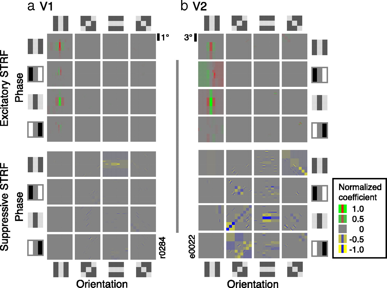
Representative STRFs for neurons in areas V1 and V2. These images are constructed by taking each BWT wavelet, multiplying it by its weighting in the rectified BWT STRF, and summing the result. Excitatory (positive; shown here in red-green) and suppressive (negative; blue-yellow) coefficients are shown separately. a, STRF for a typical V1 neuron from cluster A (subcluster A1). The STRF is a spatial map of the tuning of the neuron (only the peak temporal response latency is shown). It is separated into excitatory (red-green; top 4 × 4 panels) and suppressive components (blue-yellow; bottom 4 × 4 panels). These are further subdivided by phase (rows) and orientation (columns). Each panel represents a region encompassing three times the size of the CRF of the neuron. Top, The strongest excitatory wavelet is tuned for vertical orientation and intermediate spatial frequency, at all phases. Bottom, Several weak suppressive wavelets tuned for horizontal orientation are located both within and outside the CRF. This is a classical V1 neuron with weak cross-orientation suppression. b, STRF for a typical V2 neuron from cluster B (subcluster B2). The structure of the panel is the same as in a. Top, The excitatory tuning of this neuron is similar to that shown in a. Bottom, Suppression in this STRF is strong in multiple wavelet channels. Although the excitatory STRF of this neuron is compatible with the classical Gabor model of V1, the suppressive STRF will confer complex feature selectivity quite different from that found in V1.
Other V1 and V2 neurons in cluster A show similar classical V1 tuning. The STRFs of most of these neurons are dominated by a single excitatory wavelet channel, and they show weak suppression at 90° to the primary excitatory orientation (subcluster A1). Some neurons in this cluster have broad excitatory orientation tuning (subcluster A2), a property reported previously in both V1 (Conway, 2001) and V2 (Hubel and Livingstone, 1985; Ts'o et al., 2001).
One-half of V2 neurons are distinguished by strong suppression
Cluster B contains one-half of the V2 neurons and only a small minority of V1 neurons. The relative paucity of V1 neurons in this cluster suggests that these neurons represent properties of natural images not typically represented in V1. Figure 5b shows the STRF of a typical V2 neuron from cluster B. The strongest excitatory wavelet channel in this STRF (right-hand panel, top) is vertical, medium spatial frequency, and located within the CRF. This simple excitatory tuning profile is similar to that found in the excitatory channels of neurons in cluster A. However, the STRF of this cluster B neuron also contains several strong suppressive channels at diverse orientations and spatial frequencies, both within and outside the CRF (right-hand panel, bottom). This suppression is stronger and more widespread than is found in the neurons of cluster A (compare the V1 neuron shown in Fig. 5a). Most of the neurons in cluster B have a similar pattern of excitatory and suppressive structure: their excitatory tuning is dominated by a small number of wavelet channels and is accompanied by strong suppressive tuning from a larger number of wavelet channels. Similar patterns of suppressive tuning have been reported previously in area 18 of the cat cortex (Nishimoto et al., 2006).
These data suggest that approximately one-half of the V2 neurons incorporate strong, tuned suppression from multiple wavelet channels that is not observed in V1. To quantify this difference, we calculated an excitation index, E, for each V1 and V2 neuron. The excitation index summarizes the relative strength of excitatory and suppressive wavelet channels in each STRF (Fig. 6a, inset). The median excitation index of the V1 sample (Fig. 6a, 0.73) is significantly higher than the median of the V2 sample (Fig. 6b, 0.28) (p = 0.0042; Kruskal–Wallis one-way ANOVA; df = 141). The strength of excitatory and suppressive tuning in various subclusters in the combined V1–V2 sample is summarized in Figure 7. Together, these data confirm the substantial difference in tuned suppression between areas V1 and V2. To demonstrate that this extra suppressive tuning is genuinely tuned (rather than an artifact of nonspecific suppression as seen in Fig. 5a), we performed a number of control analyses, which are described below (see Suppression in V2 is tuned).

Excitation index, E, quantifying the relative strength of excitatory versus suppressive tuning in each neuron. Inset, E is calculated as a contrast ratio between the summed excitatory (h+) and suppressive (h−) weights assigned to the wavelets in each STRF. a, Histogram of E across the sample of 46 V1 neurons. The median (0.73) and the cell shown in Figure 5a are marked. b, Histogram of E for the sample of 96 V2 neurons. The median (0.28) and the cell shown in Figure 5b are marked. The median value of E is significantly lower in V2 than in V1 (p = 0.0042; Kruskal–Wallis one-way ANOVA; df = 141), indicating that suppression is substantially stronger in V2 than in V1. The V2 distribution is significantly non-unimodal at p = 0.002 (Hartigan's dip test using 1000 bootstraps). The V1 distribution is not significantly non-unimodal (p = 0.70). c, Distribution of E for all neurons, broken down into the clusters identified in Figure 4. Cluster B (pink, orange) contains neurons with significantly stronger tuned suppression than cluster A (cyan, purple; p ≪ 0.001, Welch's t test, df = 121). The complete V1–V2 distribution is significantly non-unimodal at p = 0.005 (Hartigan's dip test using 1000 bootstraps). d, Breakdown of excitation index by animal, for V1 neurons. e, Breakdown of excitation index by animal for V2 neurons. No significant differences in the excitation index were found for different animals in this study. f, Suppressive tuning in V2 is not caused merely by surround suppression. The rectified BWT STRF for each V2 neuron was analyzed to determine the relative contributions of the CRF and nCRF to suppressive tuning. The suppressive coefficients in each STRF were classified according to whether they were in the CRF (central square of the STRF at scale level 2) (Fig. 1b) or nCRF (surrounding squares). The coefficients in the CRF and nCRF were summed separately, and a contrast index was calculated as follows: C = (ΣhCRF − ΣhnCRF)/(ΣhCRF + ΣhnCRF). The distribution of C across the sample of 96 V2 neurons is shown here. A value of 1 would indicate that tuned suppression came purely from the CRF; a value of −1 would indicate that tuned suppression came purely from the nCRF. For most V2 neurons, the suppressive coefficients are mainly found in the CRF (values >0). This indicates that the tuned suppression we observe in V2 cannot accurately be described as surround suppression.

Mean excitatory and suppressive tuning for orientation energy of the subclusters of the combined V1/V2 sample. For each neuron, orientation tuning was estimated by summing separately the positive and negative wavelet coefficients at each orientation (0, 45, or 90°) in the corresponding STRF. Orientation tuning was then averaged across the neurons in each subcluster (A1, A2, B1, B2, as in Fig. 4). Neurons in subclusters A1 and A2 are dominated by tuning at 0° (i.e., parallel to the strongest excitatory wavelet in their STRFs) and show very little suppressive tuning. Neurons in subclusters B1 and B2 have excitatory tuning similar to those in subclusters A1 and A2, but they also have strong suppressive tuning. Suppression is strongest in subcluster B2. Error bars give the SEM.
To confirm that the V1–V2 distribution represents a genuinely bimodal distribution, rather than a continuum, Hartigan's dip test was used as a measure of non-unimodality. The overall V1–V2 distribution is significantly non-unimodal at p = 0.005, and the V2 distribution is significantly non-unimodal at p = 0.002. The V1 distribution is not significantly non-unimodal (p = 0.70). This confirms that there are two distinct clusters within the V1–V2 distribution and that this results from the presence of two distinct clusters within V2. V1, however, is relatively homogeneous.
Much of the rest of this report focuses on the functional properties of the two major clusters of V2 neurons. To facilitate discussion we refer to the V2 neurons that are functionally similar to those in V1 (cluster A) as “weakly suppressed” neurons, and those that are functionally distinct from V1 (cluster B) as “strongly suppressed.”
Increased suppression in V2 relative to V1 is not a modeling artifact
Using the rectified BWT STRF model, our sample of V2 neurons showed stronger suppressive tuning than our sample of V1 neurons (Fig. 6a–c). Since the rectified BWT is a novel model, it is possible that this result is merely an artifact of the BWT model. To ensure that this is not the case, the STRF estimation and measurement of the excitation index were repeated using numerous different STRF models (for details of all these models, see Materials and Methods).
One possibility is that our results might be an artifact of the spatial structure of the BWT filters. The BWT filters are qualitatively similar to V1 simple cells (tuned in space, spatial frequency, and orientation), but they are not perfect models of V1 receptive fields. Additionally, they do not contain any center-surround filters, even though such receptive fields are found in V1. To determine whether the spatial structure of the BWT affected our results, the data were refit using alternative models with different spatial structure. The BWT plus center-surround model supplemented a complete set of BWT filters with a set of pixelated center-surround filters. The rectified difference-of-Gaussians and rectified pixels models replaced the BWT filters with circularly symmetric filters.
Table 1, rows 2–4, shows the results of fitting the data with these alternative models. In each case, the proportion of explainable variance accounted for (in both V1 and V2) is equal to or lower than the rectified BWT model. This indicates that the spatial structure of the rectified BWT model has not adversely affected its ability to describe the behavior of V1 and V2 neurons. The values of excitation index in V1 and V2 vary somewhat from model to model. However, in all cases, there is a significant difference in excitation index between V1 and V2 (p < 0.01). This indicates that our central result—that tuned suppression is stronger in V2 than in V1—is not sensitively dependent on the spatial structure of the STRF model used.
Comparison of rectified BWT and alternative STRF models
An additional possibility is that the difference in excitation index arises because the rectified BWT model is a better model of V1 neurons than of V2 neurons. This might result in different distributions of BWT coefficients in V1 and V2, which in turn might produce differences in the excitation index between the two areas. To investigate this possibility, two measurements were made of the relationship between fit quality and excitation index. Figure 8a shows a scattergram of the total strength of negative coefficients in each kernel (h−) against the total strength of positive coefficients (h+). The total strength of coefficients indicates how many iterations the boosting algorithm has run through. Thus, if the excitation index merely depended on fit quality, one might expect to see some inhomogeneity in these distributions. Instead, the difference between V1 (open circles) and V2 (filled circles) is clear in this plot and is distributed across the range of possible values of h+ and h−, indicating that there is no systematic bias.

Measures of possible bias in the excitation index. a, Scattergram showing log of the summed negative coefficients in each rectified BWT STRF against log of the summed positive coefficients. V2 neurons (filled circles) tend to have stronger negative coefficients than V1 neurons (open circles), regardless of the overall strength of the coefficients. This indicates that the difference between V1 and V2 is not merely an artifact of overall coefficient strength (as might be expected if the model simply provided a worse fit to V2 neurons than to V1 neurons). b, Scattergram showing excitation index against prediction correlation coefficient (CC) (Pearson's r). If excitation index were an artifact of fit quality, we would expect to see a strong relationship between these two variables. In fact, we find that there is no strong relationship, indicating that the difference between excitation index in V1 and V2 is not merely an artifact of fit quality.
Figure 8b shows a scattergram of excitation index against prediction correlation coefficient. Again, if excitation index were dependent on fit quality, one would expect to see a systematic relationship here. Instead, it is clear that there is no such relationship. From these two analyses, it is clear that the excitation index effect is not an artifact of fit quality.
Increased suppression in V2 relative to V1 does not result from an inappropriate choice of output nonlinearity
In principle, it is possible that our observation of increased tuned suppression in V2 might merely result from a poor choice of output nonlinearity. If the half-wave rectification used in the rectified BWT model is inappropriate for visual neurons, the model might provide a poor fit to the neuronal responses. To determine whether this was the case, the data were refit using two alternative models. These had the same spatial structure as the rectified BWT, but used alternative output nonlinearities—rectified with positive threshold and half-squaring—which are arguably more appropriate for modeling neurons (for details, see Materials and Methods).
Table 1, rows 5 and 6, shows the results of fitting the data with these alternative models. In each case, the proportion of explainable variance accounted for (in both V1 and V2) is equal to or lower than the rectified BWT model. This indicates that the output nonlinearity used in the rectified BWT model is not inappropriate for describing the behavior of V1 and V2 neurons. The values of excitation index in V1 and V2 are similar to those for the rectified BWT model, and in all cases, there is a significant difference in excitation index between V1 and V2 (p < 0.05). For comparison, we also fit a simple linear model with no output nonlinearity (Table 1, row 7). This model is notable because it fits the data extremely poorly in both V1 and V2. This demonstrates the inadequacy of linear models for describing the responses of visual cortical neurons. Furthermore, the differences in excitation index between V1 and V2 are not significant for this model.
These comparisons demonstrate that the increase in tuned suppression in V2 is not an artifact of an inappropriate choice of output nonlinearity. On the contrary, half-wave rectification describes the neuronal data just as well as other plausible nonlinearities. More importantly, the difference in excitation index between V1 and V2 is robust, so long as the model contains some output nonlinearity.
Suppression in V2 is tuned
Our results demonstrate that V2 neurons show more suppression than V1 neurons. There are three possible explanations for this increase in suppression. First, V2 neurons might have higher response thresholds than V1 neurons. Alternatively, V2 neurons might show stronger nonspecific suppression than V1 neurons. Both of these hypotheses would suggest that the tuning of V2 neurons differs quantitatively but not qualitatively from tuning in V1. A more interesting hypothesis is that the increase in suppression results from the presence of suppressive mechanisms in V2 that are tuned for specific aspects of the spatial structure of natural images. This would suggest that the tuning of V2 neurons is qualitatively different from the tuning of V1 neurons. To determine which of these hypotheses is correct, the STRF estimation was repeated using STRF models that incorporate a variable threshold and nonspecific suppression.
To test whether the increase in suppression in V2 neurons simply reflects an elevated response threshold, two models were compared: the standard rectified BWT model and a logistic model that incorporates a soft threshold. The logistic model is identical with the rectified BWT model, except that instead of the half-wave rectified linear output nonlinearity, it uses a logistic output nonlinearity. The logistic is a sigmoid function, which provides a generally accepted model of a neuron that has a response threshold at low activation values, and saturates at high activation values. By scaling and translating the logistic function, it can be used to accurately model neurons with a wide variety of different response nonlinearities. This includes (but is not limited to) neurons with half-squaring output nonlinearities and neurons with varying thresholds.
If the difference between V1 and V2 merely reflected differences in the neural response threshold (or other differences in the shape of the output nonlinearity), the logistic model would explicitly fit these differences. Thus, if this hypothesis was correct, the logistic model would provide better predictions of neural responses while using fewer suppressive wavelet channels than the rectified BWT model. In fact, the logistic model produces similar STRFs to the rectified BWT model, provides similar predictions (r = 0.39 in V1; r = 0.30 in V2) (Table 1, row 8), and results in similar differences in excitation index between V1 and V2 (p = 0.001; Kruskal–Wallis one-way ANOVA; df = 141). This indicates that the apparent increase in suppression in V2 does not merely reflect higher response thresholds in V2 relative to V1.
Alternatively, it is possible that the apparent increase in suppression in V2 relative to V1 reflects relatively stronger contrast normalization (Heeger, 1992; Carandini and Heeger, 1994). To evaluate this possibility, two variants of the rectified BWT STRF model were compared: a contrast normalized model, in which each image was contrast-normalized before being input to the BWT model; and a contrast filter model, in which a single contrast filter (whose output was equal to the SD of the images) was added to the bank of BWT filters. If the increased suppression in V2 merely resulted from an increase in contrast normalization, the STRFs produced by the contrast normalized and contrast filter models should provide better predictions of neural responses than the rectified BWT model, and the difference in excitation index between V1 and V2 should decrease. In fact, neither of these models produces better predictions than the rectified BWT model. In both cases, the difference in excitation index does decrease; this suggests that nonspecific suppressive mechanisms may be stronger in V2 than in V1. However, both models continue to show a significant difference in excitation index between V1 and V2 at p < 0.05 (Table 1, rows 9 and 10). This indicates that the increase in suppression in V2 does not merely reflect a stronger contrast normalization mechanism in V2 relative to V1 and suggests that the suppressive mechanisms in V2 are tuned for specific spatial features present in natural images.
Another possibility is that the increased suppression in V2 is the result of a surround suppression mechanism (DeAngelis et al., 1994). To determine whether surround suppression is responsible for the difference in excitation index between V1 and V2, the distribution of suppressive coefficients in the CRF and nonclassical RF (nCRF) was measured. The majority of the suppressive coefficients in the STRFs are located in the CRF, not the nCRF (Fig. 6f), indicating that the suppressive mechanism in V2 cannot accurately be described as surround suppression.
These control analyses indicate that the increase in suppression in V2 does not merely result from an increase in the mean response threshold of V2 neurons, or from an increase in the strength of nonspecific suppressive mechanisms that are known in V1. This strongly suggests that the observed increase in suppression is the result of tuned suppressive mechanisms in V2 that are selective for specific spatial features present in natural images.
Suppressive tuning in V2 confers selectivity for higher-order image structure
The STRFs that we have estimated here provide an objective, quantitative model of the way that V2 neurons integrate visual information. However, the STRFs alone do not reveal which specific aspects of natural images are represented in V2. To address this issue, we developed a procedure that enabled us to separately visualize the stimulus properties that tend to excite and suppress each neuron. The BWT STRFs were first decomposed into two separate hyperchannels: one containing all of the excitatory channels and one containing all of the suppressive channels. These hyperchannels were then used to filter a large set of natural images (n = 40,000). Finally, the images predicted to be excitatory and suppressive for each neuron were aggregated into summary plots.
Figure 9a summarizes the result of this analysis for the V1 neuron whose STRF is shown in Figure 5a. The horizontal axis represents the response of the excitatory hyperchannel, and the vertical axis represents the response of the suppressive hyperchannel. A small subset of images has been projected onto the plot to illustrate which images are predicted to evoke stronger or weaker responses from the excitatory and suppressive hyperchannels. This neuron has a strong excitatory hyperchannel that is activated by images containing vertical structure (right-hand side) and a weak suppressive hyperchannel that is activated by images containing horizontal structure (top). The predicted response of the neuron is equal to the difference between the activation of the excitatory and the suppressive hyperchannels. This is shown by diagonal lines and by shading indicating the overall response strength. The neuron should respond most strongly to images that activate the excitatory hyperchannel and do not activate the suppressive hyperchannel (bottom right; yellow and red regions). Since the suppressive hyperchannel is relatively weak for this neuron, most images lie toward the bottom of the y-axis, indicating that they only weakly activate the suppressive hyperchannel. Thus, this V1 neuron should respond fairly strongly to any image containing vertical structure that matches its excitatory hyperchannel, and most images are predicted to elicit some response (top left; blue region).

Functional consequences of suppressive tuning in V1 and V2. a, The STRF of a typical V1 neuron from cluster A1, decomposed into separate excitatory and suppressive hyperchannels. The x-axis quantifies the response of the excitatory hyperchannel and the y-axis the suppressive hyperchannel. Red, yellow, and blue regions identify the images that elicit strong, medium, and no responses from the neuron, respectively. Each hyperchannel was used to filter 40,000 natural images. A subset of the images is plotted according to the responses of the hyperchannels. The excitatory hyperchannel of this neuron (x-axis) is vertically tuned, and so responds to any image containing vertical structure (observe the variety of images in rightmost columns). The suppressive hyperchannel (y-axis) is weakly tuned for horizontal structure. This channel suppresses responses to images that contain horizontal structure, so the neuron responds more strongly to isolated vertical edges (red region) than to complex images containing vertical and horizontal structure (yellow region). However, these suppressive effects are weak in V1 and in the weakly suppressed neurons in V2. b, Similar decomposition of the STRF of a typical strongly suppressed V2 neuron. The excitatory hyperchannel (x-axis) of this neuron is also tuned for vertical structure, and the suppressive hyperchannel (y-axis) is tuned for horizontal structure. In this neuron, the suppressive hyperchannel is much stronger than the one shown in a. Therefore, many more images produce only weak or zero responses (compare the number of images in the blue and white regions in Fig. 9a,b). A smaller proportion of images are in the yellow and red regions in Figure 9b than in Figure 9a, indicating that tuned suppression has increased the selectivity of the V2 neuron relatively to the weakly suppressed neuron in a.
Figure 9b shows the same analysis for a typical strongly suppressed V2 neuron (cluster B). As for the V1 neuron shown in Figure 9b, the excitatory hyperchannel of this neuron is tuned for vertical structure and the suppressive hyperchannel is tuned for horizontal structure. However, the suppressive hyperchannel is approximately twice as strong here as in Figure 9a. (Compare the many images toward the top of Fig. 9b vs the number in similar locations in Fig. 9a.) This neuron is predicted to respond only to those specific images containing vertical structure, as long as they activate the excitatory hyperchannel and do not activate the suppressive hyperchannel. As a result, a smaller proportion of images produce strong responses (bottom right; yellow and red regions), and there are many more images that fail to produce any overall activation (top left; blue region).
For both the V1 neuron (Fig. 9a) and the V2 neuron (Fig. 9b), images that contain only vertical structure should activate the excitatory hyperchannel and produce strong responses (red region). Images that contain some horizontal structure will also elicit strong responses from the V1 neuron (yellow region), because this neuron does not possess a substantial suppressive hyperchannel. However, images that contain horizontal structure will elicit only a weak response from the V2 neuron (white region), because those images will activate the strongly suppressive hyperchannel. Thus, whereas the V1 neuron is tuned for vertical energy, the V2 neuron is tuned for a specific configuration of oriented elements. In order for the V2 neuron to respond strongly, some wavelet elements must be present (those that match the excitatory hyperchannel) and others must be absent (those that match the suppressive hyperchannel).
The maps shown in Figure 9 suggest that many more stimuli are likely to elicit a strong response from the weakly suppressed V1 neuron than from the strongly suppressed V2 neuron (compare proportion of stimuli falling in yellow and red portions of Fig. 9a,b). This pattern suggests that suppression serves to increase stimulus selectivity and reduce the range of stimuli that will elicit a robust response. Thus, weakly suppressed neurons tend to function as simple feature detectors for images whose spectral structure matches the excitatory hyperchannel. In contrast, strongly suppressed neurons are selective for a specific combination of features.
The pattern of suppression observed across the entire sample of strongly suppressed V2 neurons is diverse, even after normalizing for the primary excitatory orientation. This suggests that suppression increases both the complexity and diversity of stimulus features that modulate responses of strongly suppressed neurons in area V2, relative to V1 (Hegdé and Van Essen, 2000; Ito and Komatsu, 2004).
Frequency pooling in V2 may support illusory contour selectivity
Previous research has shown that many V2 neurons are selective for illusory contours (von der Heydt et al., 1984; von der Heydt and Peterhans, 1989). One way to build an illusory contour-sensitive neuron in V2 would be to pool the rectified output of many V1 neurons with different preferred spatial frequencies but a single preferred orientation. By nonlinear summation of oriented structure beyond the CRF, such a neuron could respond to an extended contour even if the part of the contour within the CRF was missing. Some of the neurons that we observed in cluster B do appear to pool information across spatial frequency at a single orientation (Fig. 10). In the neurons that have this property, frequency pooling often spans several octaves. Frequency pooling in V2 suggests that illusory contour selectivity in this area is conferred by a general mechanism whose function is to reliably represent edges in natural scenes. Natural edges are composed of a broadband distribution of phase-aligned frequency elements at a single orientation. The V2 neurons whose receptive field profile matches natural edge structure are likely to form a more reliable and explicit representation of edges than can be achieved by the narrowband Gabor filters in V1.

STRF of one V2 neuron that pools across spatial frequency. The excitatory STRF of this neuron (top 4 rows) is tuned for horizontal orientation at several spatial scales (and so several spatial frequencies), both within and beyond the CRF. A mechanism that pools information at a single orientation, but across spatial position and spatial scale, may confer selectivity for both real and illusory contours in natural images.
Discussion
Using an unbiased natural stimulus set and nonlinear system identification analysis, we have shown that area V2 is divided into two functionally distinct subpopulations: one whose spatial tuning characteristics are functionally similar to area V1, and one that is functionally distinct. Both V1 and V2 neurons have similar excitatory spatial tuning profiles, but the functionally distinct V2 neurons (approximately one-half of the sample) have strong suppressive spatial tuning rarely seen in V1.
Functional significance of tuned suppression in V2
Previous studies that used sinusoidal gratings suggested that tuning in V2 is fundamentally similar to that found in V1 (Levitt et al., 1994); other studies using complex stimuli (von der Heydt et al., 1984; von der Heydt and Peterhans, 1989; Hegdé and Van Essen, 2000; Zhou et al., 2000; Ito and Komatsu, 2004) suggested that V2 neurons are functionally distinct from those in V1. Our experiment resolves this longstanding controversy by demonstrating that neither extreme view is correct: V2 is functionally heterogeneous, just as it is anatomically heterogeneous (Sincich and Horton, 2002). This is consistent with the findings of one other recent study of V2 (Anzai et al., 2007). Note, however, that our experiments did not investigate all stimulus dimensions to which V2 neurons are sensitive [e.g., binocular disparity (Thomas et al., 2002) and color (Lu and Roe, 2007)]. Additional studies will therefore be required to determine whether the subpopulation of V2 neurons that appears to be functionally similar to those found in V1 can be distinguished along some other dimension that was not examined in our experiment.
The functional role of tuned suppression is inherently difficult to interpret, because suppression reduces neural responses. Our analysis suggests that the primary function of suppression in V2 is to provide an explicit representation of spatial configurations of features that are not represented explicitly in V1. Although neurons in both V1 and V2 will respond to a single Gabor wavelet presented in isolation, only the strongly suppressed V2 neurons can reliably distinguish between images containing the same wavelet in different contexts. Recall that any natural image can be viewed as the linear sum of many sparsely distributed Gabor wavelets (Field, 1994). Under natural viewing conditions the responses of both V1 neurons and the weakly suppressed V2 neurons will be primarily determined by the probability that the sparse components of each natural image (i.e., the constituent Gabor wavelets) match the excitatory components of the STRF. In contrast, the responses of strongly suppressed V2 neurons will be determined by the joint probability of occurrence of a few excitatory Gabor wavelets and all of the many Gabor wavelets that match the suppressive components of the STRF. We speculate that the structure of the suppressive components of these receptive fields are optimized to match the higher-order statistics of natural scenes (Geisler et al., 2001).
The STRFs we have estimated for V2 neurons provide a quantitative functional model of how complex stimulus selectivity in V2 (von der Heydt and Peterhans, 1989; Hegdé and Van Essen, 2000; Ito and Komatsu, 2004) is constructed by combining the relatively simple receptive fields found in V1. Selectivity for complex features in single V2 neurons is not simply the result of excitatory pooling over many V1 neurons. Instead, each V2 neuron combines excitatory pooling from a relatively small number of similar V1 neurons with suppressive pooling from much larger and more diverse set of V1-like subunits. Our findings are consistent with studies of other sensory areas that have suggested that inhibitory interneurons and synaptic depression play a critical role in determining neuronal tuning (Freeman et al., 2002; Wehr and Zador, 2003). Many current computational theories of vision emphasize the role of excitatory feedforward connections between cortical areas (Riesenhuber and Poggio, 1999; Serre et al., 2007). Our data show the importance of incorporating tuned suppression into future models.
Effect of model structure
In this study, we fit a variety of nonlinear STRF models to the same data set and compared the fits provided by these models. Comparison of these fits raises two issues for modeling visual neurons. First, it demonstrates the importance of nonlinearity in modeling visual neurons. Of the models we used, the linear model provides by far the worst predictions of neural behavior in both V1 and V2. Similarly, the linear model is the only model that does not show a significant difference in excitation index between V1 and V2.
Second, this comparison shows that the spatial structure of the filters used in the STRF model is relatively unimportant. All of the nonlinear models provided reasonable predictions of V1 and V2 responses. Similarly, differences in excitation index between V1 and V2 were consistent, regardless of the set of the model used. This suggests that building nonlinear models of visual neurons may not be as difficult as is generally assumed. It is not necessary to use a truly biologically accurate model, because many plausible models will provide good descriptions of neural behavior.
Natural stimuli
In this study, we investigated neural behavior using natural stimuli. Such stimuli present serious challenges for neurophysiology experiments. First, they have complex correlational structure that must be accounted for when calculating STRFs. The BWT STRF model used here solves this problem by providing a computationally efficient way of estimating accurate STRFs despite the presence of stimulus correlations.
An additional problem arises because natural stimuli have very high dimensionality. In a typical experiment using grating stimuli, the gratings vary along only a few dimensions (spatial frequency, orientation, etc.). As a result, most of the tuning space of a neuron (and therefore its response variance) is not explored by such experiments. In contrast, the natural scenes used in this experiment have very high dimensionality (they were typically shown at 128 × 128 pixels, giving 216,384 dimensions, although stimulus correlations reduce their effective dimensionality). As a result, natural scenes probe a large portion of the space of a neuron, and of its response variance. Producing a model that can accurately describe the responses of the neuron throughout this high-dimensional space is challenging, and this is reflected in the relatively low prediction scores obtained by all the models in this study.
Natural stimuli also have important advantages for understanding the behavior of sensory neurons. For example, it is difficult to observe the interaction between excitation and suppression without using natural stimuli. Simple stimuli such as sinusoidal gratings are likely to stimulate neurons only in simple ways (i.e., they may produce excitation without suppression or suppression without excitation). It is only by using complex stimuli that we can stimulate excitatory and suppressive channels simultaneously, and thereby investigate the interactions between excitation and suppression. Natural stimuli evoke ecologically relevant patterns of excitation and suppression, for which neurons are likely to be tuned. Complex, natural stimuli therefore provide an ideal way to uncover these subtle interactions.
To understand how the brain represents and processes visual input outside the laboratory, it is essential to understand the response of neurons to natural stimuli. However, natural stimuli are inevitably complex and so it is difficult to use them in controlled neurophysiological experiments. The nonlinear system identification approach used here can overcome many of the drawbacks of using natural images (Wu et al., 2006). Most importantly, nonlinear system identification provides an objective and quantitative procedure for modeling the stimulus–response relationship in terms of an explicit, biologically plausible model (in this specific case, the Berkeley wavelet transform). This general approach can also be applied to higher visual areas. For example, it could be used to understand how the neural representations in areas V4 and IT are constructed by excitatory and suppressive combination of the nonlinear outputs of neurons in V1 and V2. Our results suggest that functional characterization of higher-order visual neurons will be facilitated by the use of complex, naturalistic stimuli, combined with quantitative nonlinear system identification analysis.
Footnotes
-
This work was supported by National Eye Institute and National Institute of Mental Health. Statistical guidance was kindly provided by B. Yu. The neurophysiology software was written by J. A. Mazer, and the database system was written by S. V. David.
- Correspondence should be addressed to Jack L. Gallant, Psychology Department, University of California, Berkeley, 3210 Tolman Hall, #1650, Berkeley, CA 94720-1650. gallant{at}berkeley.edu.


